An introduction to statistics in R
A series of tutorials by Mark Peterson for working in R
Chapter Navigation
- Basics of Data in R
- Plotting and evaluating one categorical variable
- Plotting and evaluating two categorical variables
- Analyzing shape and center of one quantitative variable
- Analyzing the spread of one quantitative variable
- Relationships between quantitative and categorical data
- Relationships between two quantitative variables
- Final Thoughts on linear regression
- A bit off topic - functions, grep, and colors
- Sampling and Loops
- Confidence Intervals
- Bootstrapping
- More on Bootstrapping
- Hypothesis testing and p-values
- Differences in proportions and statistical thresholds
- Hypothesis testing for means
- Final thoughts on hypothesis testing
- Approximating with a distribution model
- Using the normal model in practice
- Approximating for a single proportion
- Null distribution for a single proportion and limitations
- Approximating for a single mean
- CI and hypothesis tests for a single mean
- Approximating a difference in proportions
- Hypothesis test for a difference in proportions
- Difference in means
- Difference in means - Hypothesis testing and paired differences
- Shortcuts
- Testing categorical variables with Chi-sqare
- Testing proportions in groups
- Comparing the means of many groups
- Linear Regression
- Multiple Regression
- Basic Probability
- Random variables
- Conditional Probability
- Bayesian Analysis
Approximating with a distribution model
18.1 Load today’s data
Start by loading today’s data. If you need to download the data, you can do so from these links, Save each to your data directory, and you should be set.
- Roller_coasters.csv
- Data on the height and drop of a sample of roller coasters.
# Set working directory
# Note: copy the path from your old script to match your directories
setwd("~/path/to/class/scripts")

# Load data
rollerCoaster <- read.csv("../data/Roller_coasters.csv")
18.2 Introduction
You may have noticed by now that a lot of the distributions we’ve made look rather similar to each other, especially if we ignore the scale. For example, all of these plots are:
- Unimodal (one hump), and
- Symmetrical (or roughly so)
and follow roughly the same pattern.
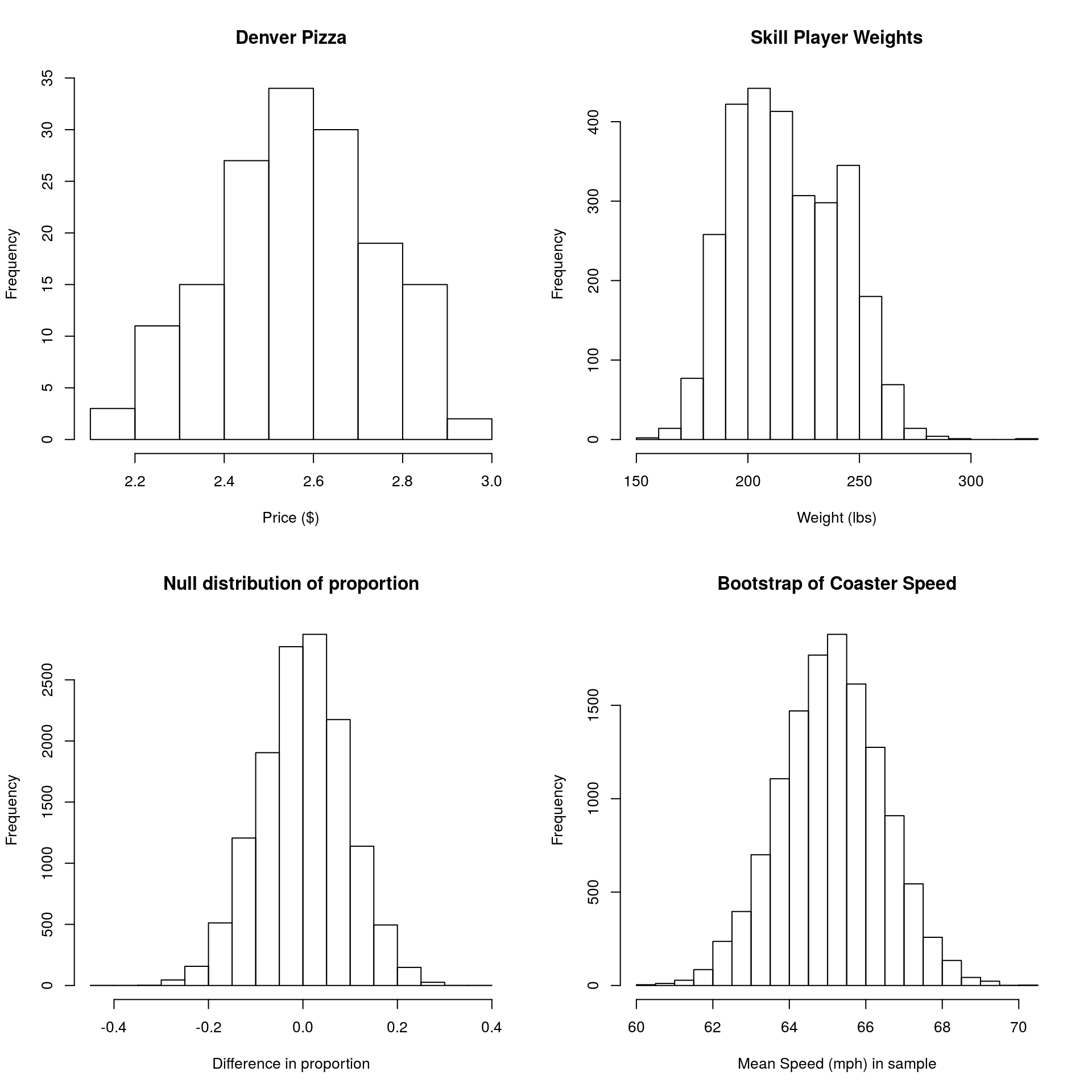
This shape has some special properties, and we are going to utilize them for the rest of the semester. In particular, the shape allows us to easily calculate the portion of data in a particular region, even if we don’t have the deep sampling we’ve been using with bootstrapping (e.g., for things from a small real world sample). These methods were originally designed to compenstate for the fact that bootstrapping and null distribution sampling wasn’t possible. However, the tools remain common and useful (at least for now).
First, I am going to superimpose a “Normal” curve on each of the plots, then we will walk through some of the advantages and things we can do with that information. Note that the axis is changing from “Frequency” to “Density”.
The density is set such that the area under the curve equals 1, which allows us to ask about the area in a particular region, which is the same as the proportion of the data in that region.
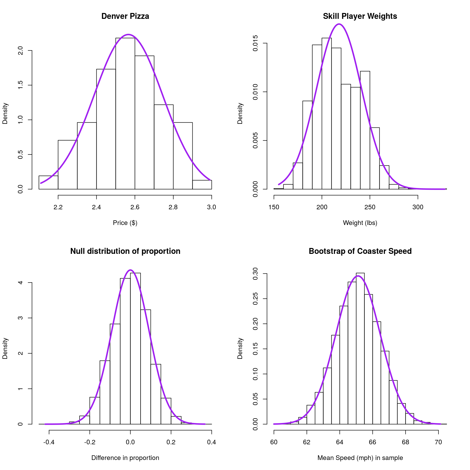
The first thing that you will notice is that, for each, the normal model is a pretty decent fit. Not bad considering that the only information used to set it is the mean and standard deviation of the data we plotted. The second thing you will likely notice is that it is almost never perfect. This is a good point to note this favorite quote of mine:
All models are wrong, but some are useful. (George Box)
The point here is that the normal, like other models, can be slightly inaccurate, but it is still a useful approximation. It gets us “close enough,” especially under conditions that we will explore more deeply.
18.3 What is the normal model
The normal distribution is a bell-shaped curve, centered at a mean value (μ) with a width governed by its standard deviation (σ).
We have already been using this model, without knowing it, when we applied the 95% rule. In any normal distribution, 95% of the values are expected to fall within 2 sd’s of the mean.
Changing the mean just shifts the distribution left or right, and changing the sd make it skinny or fat.
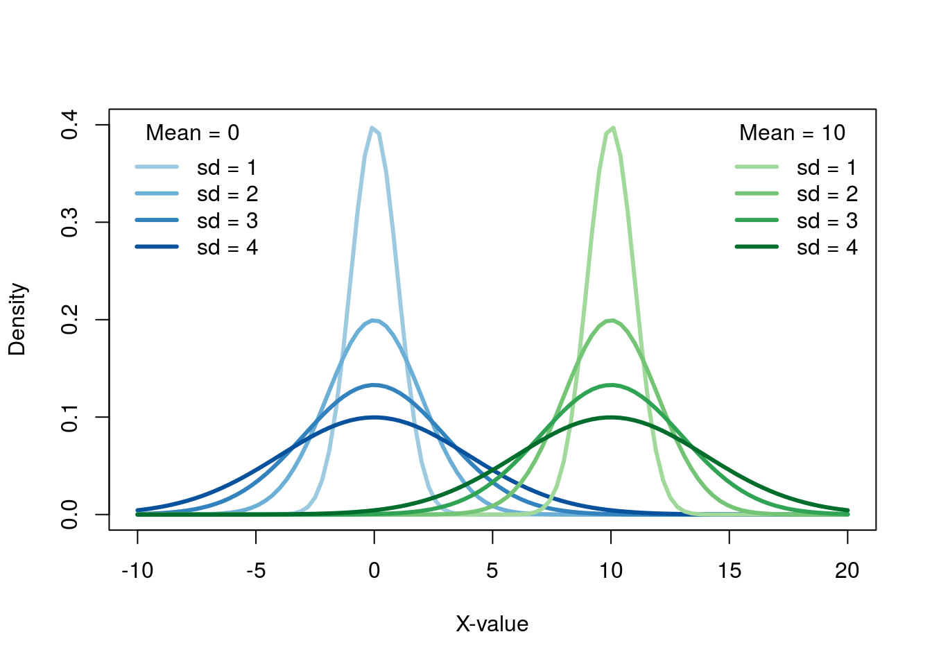
Importantly though, no matter the mean or standard deviation, the shape is always the same. While in the previous plot, the the curves with different standard deviations looked different, that is only because of scale. If we put each plot on it’s own axis, we can see this more clearly.
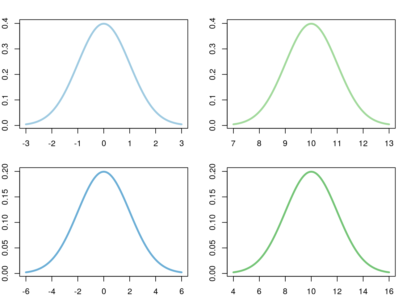
Note that, in the above, the scale on the x-axis is different for each plot. For each, it is centered at the mean, and each tick mark is one standard deviation. This similarity, and the fact that the standard deviation is such a useful ruler, make the normal model great for approximations as it does not matter what scale the data is on.
18.4 Drawing normal curves
In this chapter, we will focus on drawing a few of these curves. This will give you a chance to see the distribution a few times, the ability to draw it when you need it, and hopefully a sense of the normal model itself.
18.4.1 A new plotting tool
The function curve() draws a line on a plot, starting on the x-asis at the from = value and going to the to = value. It calculates y values from the function we give it. The function creates a large number of x values along the range we give it, then calculates a y value for each and connects them as a line. For example, we can plot the line y = x * 2:
# Plot simple function
curve(x*2,
      from = 0,
      to = 10)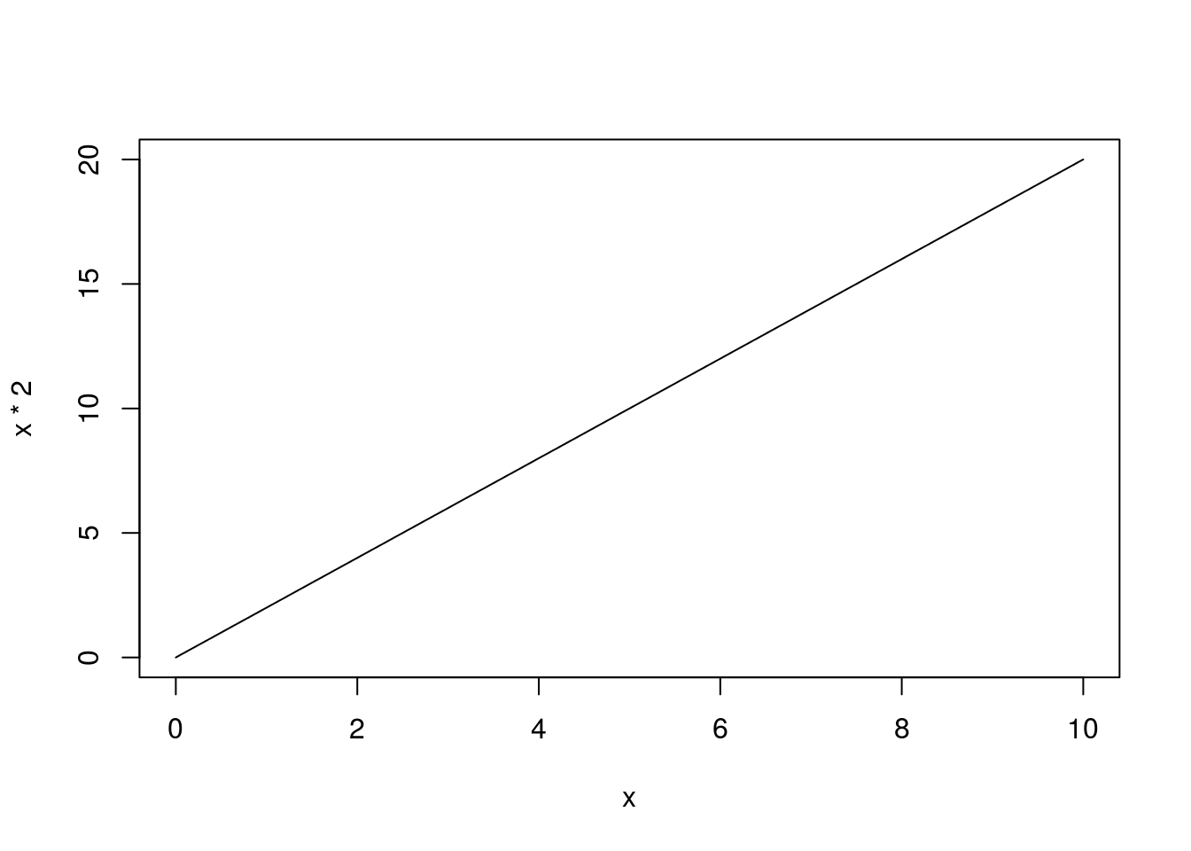
We can build more complex expressions as well. Here, we can draw a parabola
# Plot parabola
curve(x^2,
      from = -10,
      to = 10)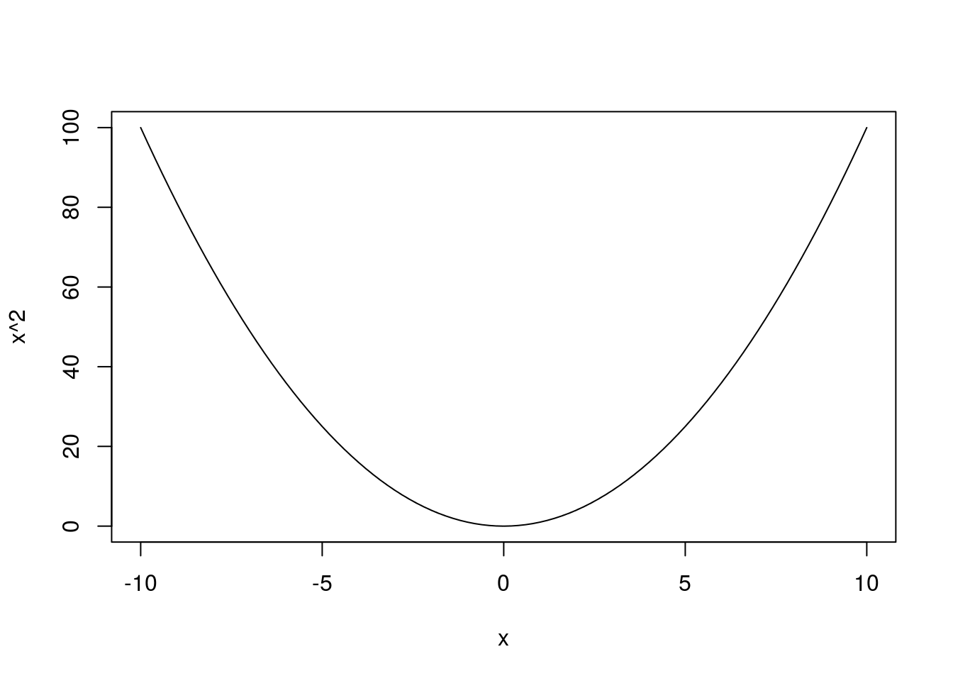
or even a complicated multinomial function:
# Plot complicated line
curve(2*x^3 + 3*x^2 - 2,
      from = -10,
      to = 10)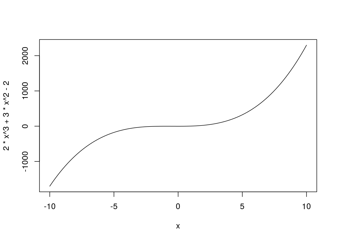
This is great for plotting lines, but it doesn’t help us plot a normal curve.
18.4.2 Calculating densities
What we need is a function to produce the density of a normal distribution. In R, this is dnorm() which returns the density of a normal distribution, at the points given. For example.
# Show the denisty of a normal curve
dnorm(-2:2)
## [1] 0.05399097 0.24197072 0.39894228 0.24197072 0.05399097But, we have said a few times that the normal curve is specified with a mean and a standard deviation. dnorm() (and other functions like it) uses default values of mean = 0 and sd = 1, which are often referred to as the “standard normal” distribution (just like the z-scores we calculated earlier). However, we can set a different mean to get the density of any normal curve.
# show density of a different curve
dnorm(8:12,mean = 10)
## [1] 0.05399097 0.24197072 0.39894228 0.24197072 0.05399097# show density of a different curve
dnorm(8:12,mean = 10, sd = 2)## [1] 0.1209854 0.1760327 0.1994711 0.1760327 0.1209854We can, in this way, generate the density of any normal distribution that we want. Putting it together curve(), we can then plot that distribution.
# Plot a standard normal distribution
curve(dnorm(x),
      from = -3,
      to = 3)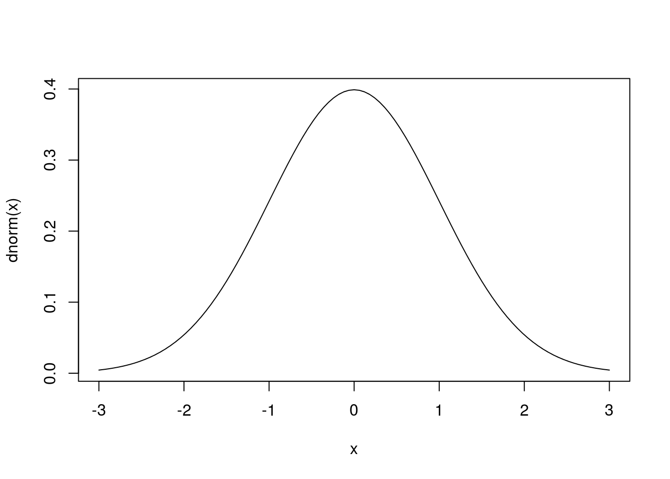
By setting a different mean = and sd =, we can draw a different normal model.
# Plot a different normal distribution
curve(dnorm(x, mean = 10, sd = 2),
      from = 4,
      to   = 16)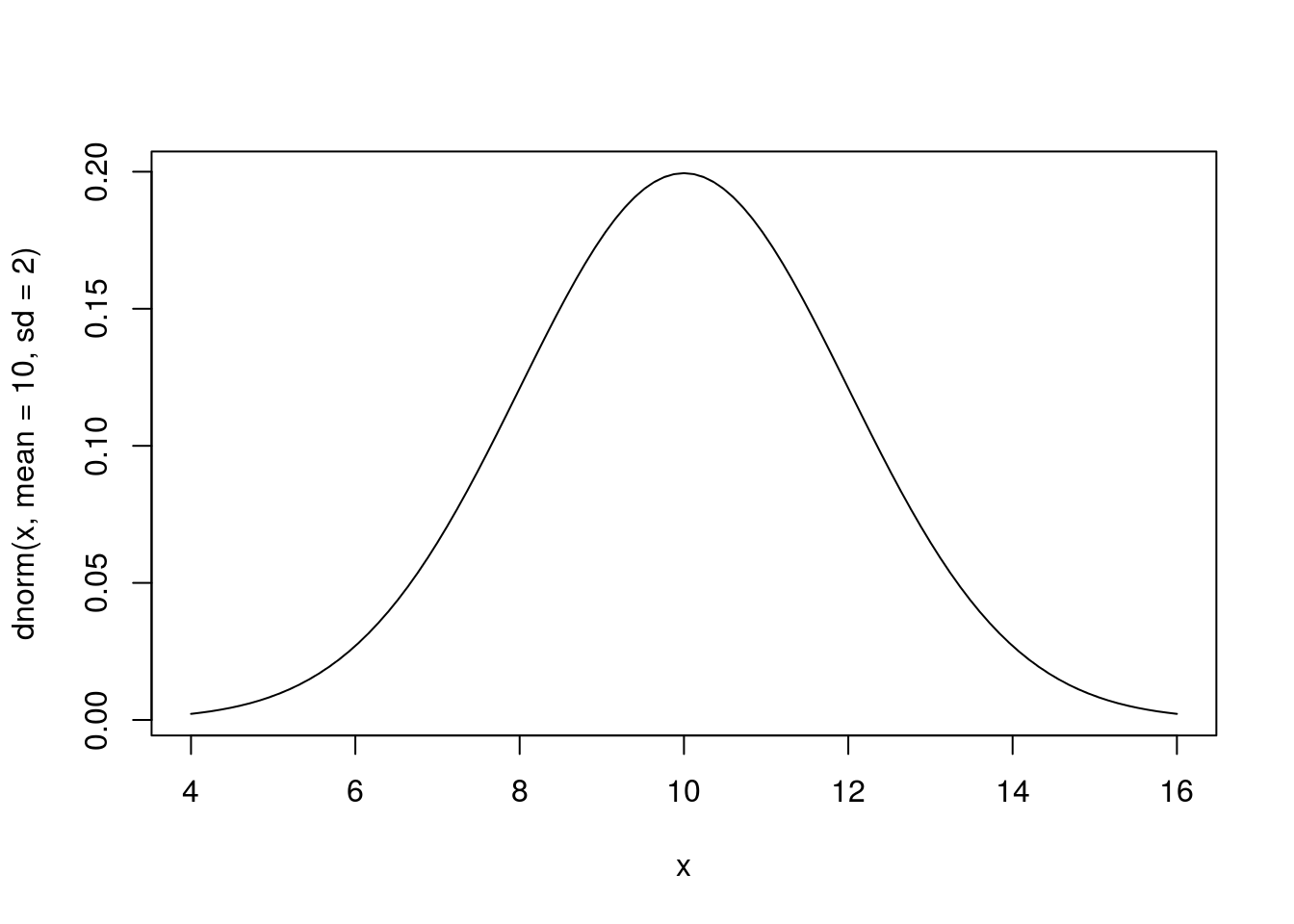
What changed between these two plot? Notice the from = and to = arguments above. Think carefully about what that difference means.
The function curve also accepts a number of other arguments, including the ylab =, col = and lwd = options we’ve used extensively before.
# Plot a different normal distribution
curve(dnorm(x, mean = 10, sd = 2),
      from = 4,
      to   = 16,
      col = "purple", lwd=3,
      ylab = "Density")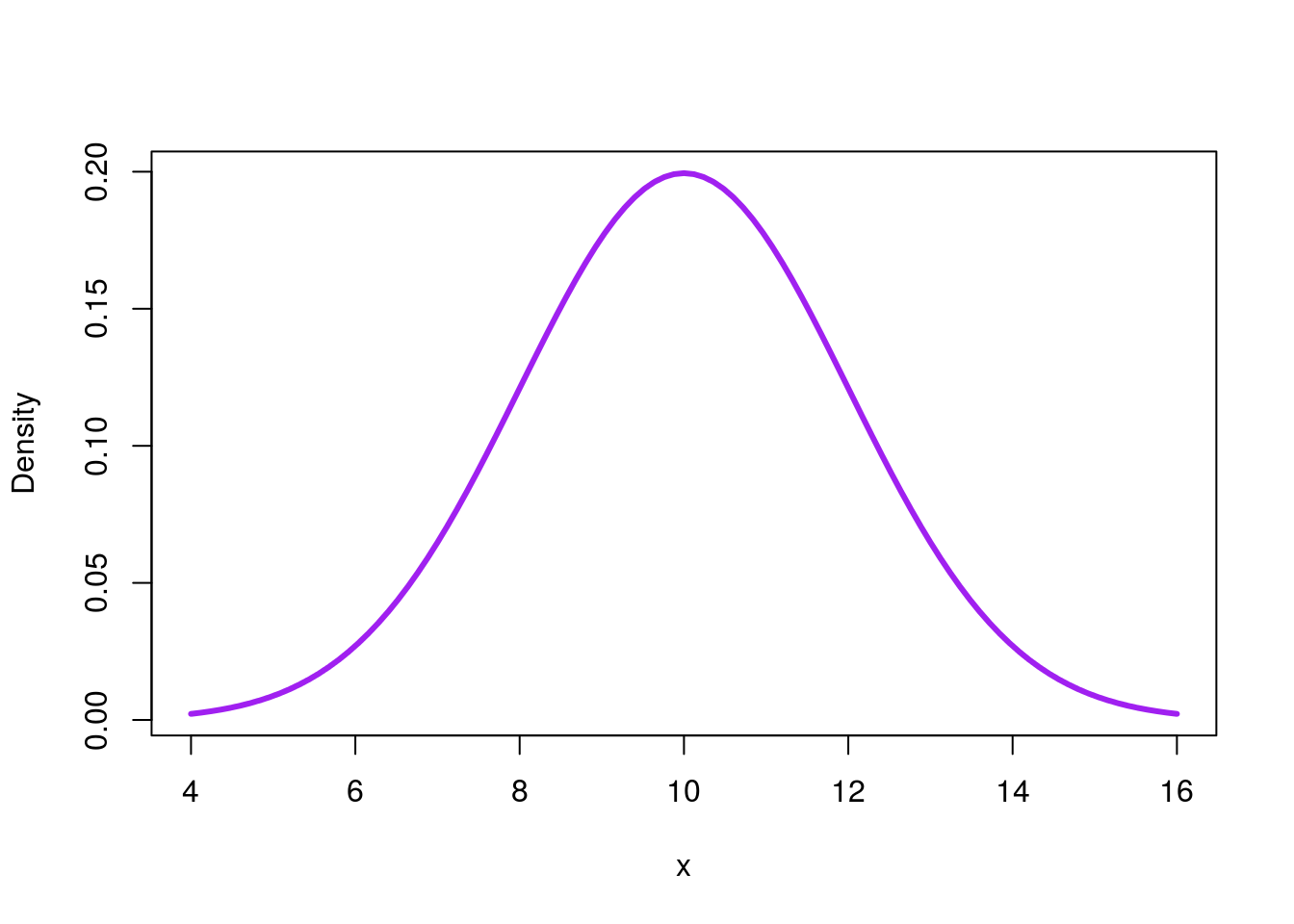
18.4.2.1 Try it out
Use the above code to draw at least 3 different normal curves. What differences do you notice between them?
18.4.3 Drawing with real data
First, let’s generate something with a nice, unimodal, symmetric, shape. Copy in the following to generate a bootstrap distribution of the speed of roller coasters (we also did this in an earlier lesson).
# Coaster bootstrapping

# Initialize vector
coasterBoot <- numeric()

# Loop through many times
for(i in 1:12489){
  # calculate the correlation
  # note, we could save these each as a vector first
  # but we don't need to
  coasterBoot[i] <- mean(sample(rollerCoaster$Speed,
                                replace = TRUE)
                         )
}

# Plot the result
hist(coasterBoot,
     freq = FALSE,
     main = "Bootstrap of Coaster Speed",
     xlab = "Mean Speed (mph) in sample")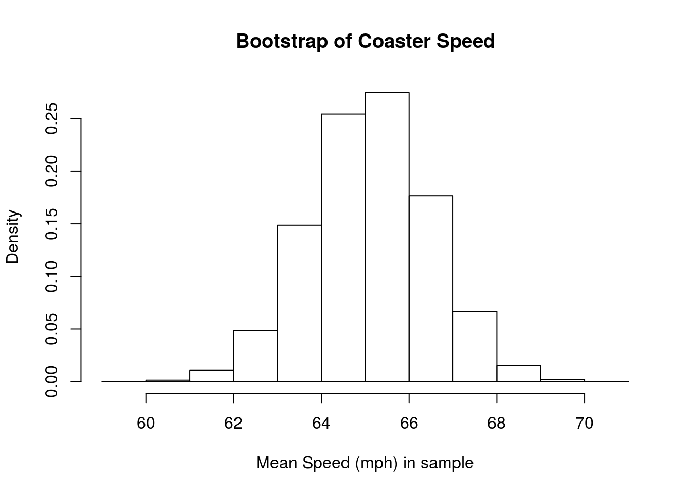
Now, let’s plot the normal curve of our coaster bootstrap. All we need to do is pass in our mean and sd, and the function does the rest. Because we are copying the bootstrap distribution, we just use the mean and standard deviation from our samples. Note that I set the from = and to = to match the range of the data. This range ensures that we can see the relavant part of the curve.
# Plot the coaster bootstrap distribution
curve(dnorm(x,
            mean = mean(coasterBoot),
            sd   =   sd(coasterBoot)),
      from = min(coasterBoot),
      to   = max(coasterBoot),
      col = "purple",
      lwd = 3,
      ylab = "Density",
      xlab = "Sample mean speed (mph)")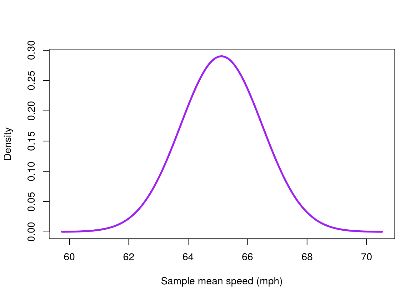
This gets us a good part of the way there, and we could use this as is. However, we can do one better, and why shouldn’t we? Let’s lay the curve on top of our histogram.
Almost all of the plotting functions in R include an option to add the plot to the existing plot, instead of overwriting it. You can use this by setting add = TRUE in most functions, including in curve.
A few notes are necessary here. First, we need to set freq = FALSE in the histogram to make sure the density is plotted. If you don’t, curve() will draw a line that looks very much like 0 (because the densities are so much smaller than counts). In addition, when using add = TRUE, it isn’t necessary to set the from = and to = options. Instead, curve() automatically matches the range of the plot.
# Plot the result
hist(coasterBoot,
     freq = FALSE,
     main = "Bootstrap of Coaster Speed",
     xlab = "Mean Speed (mph) in sample")

# Plot the coaster bootstrap distribution
# Add a curve to the plot
curve(dnorm(x,
            mean = mean(coasterBoot),
            sd   =   sd(coasterBoot)),
      col = "purple", lwd=3,
      add = TRUE)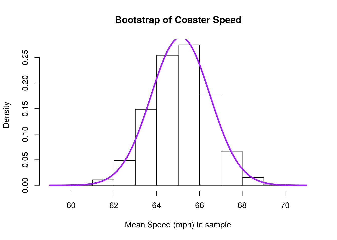
As before, we see that the curve is a very close fit to our observed data. Sometimes if the curve looks like a bad fit, it can be caused by having a poorly chosen number of bins in your histogram. Recall that we can change the number of bins by setting the breaks = argument to histogram. Thus, this plot:
# Plot the result
hist(coasterBoot,
     breaks = 60,
     freq = FALSE,
     main = "Bootstrap of Coaster Speed",
     xlab = "Mean Speed (mph) in sample")

# Plot the coaster bootstrap distribution
# Add a curve to the plot
curve(dnorm(x,
            mean = mean(coasterBoot),
            sd   =   sd(coasterBoot)),
      col = "purple", lwd=3,
      add = TRUE)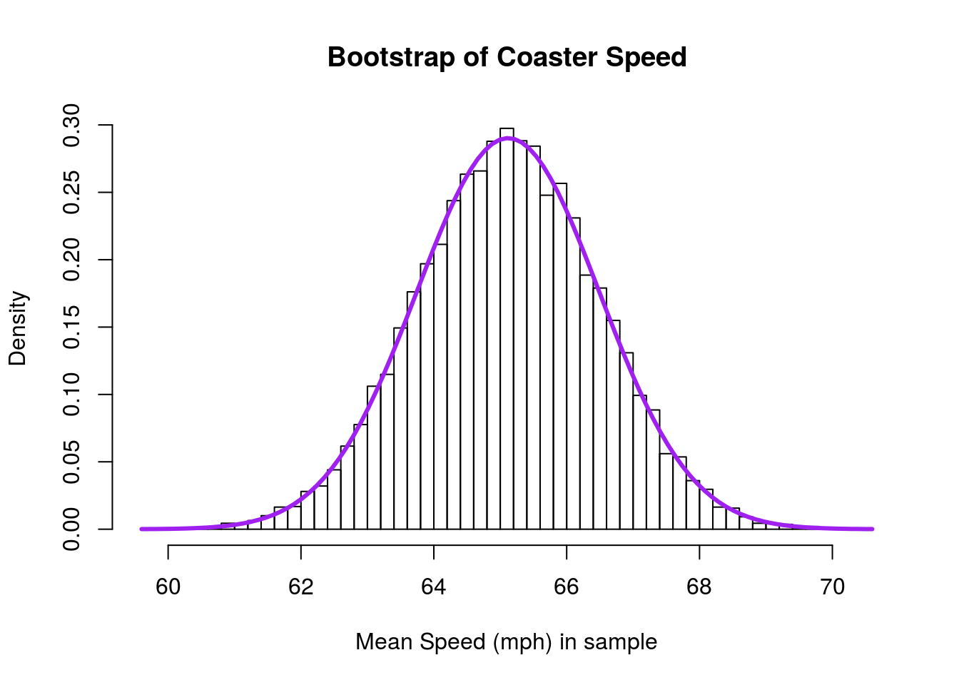
… looks like an even better fit to the normal model, despite being from the same data.
Now that we can see the distribution, we will start using these together for a few additional approaches to statistical testing.
18.4.3.1 Try it out
Go back to an earlier chapter or script and select one of the bootstrap, null, or sampling distributions. Paste the code into your script for this chapter, then plot the histogram with a curve on top of it. (Note that you may need to read the data in as well.)
How closely does the curve match your histogram?