An introduction to statistics in R
A series of tutorials by Mark Peterson for working in R
Chapter Navigation
- Basics of Data in R
- Plotting and evaluating one categorical variable
- Plotting and evaluating two categorical variables
- Analyzing shape and center of one quantitative variable
- Analyzing the spread of one quantitative variable
- Relationships between quantitative and categorical data
- Relationships between two quantitative variables
- Final Thoughts on linear regression
- A bit off topic - functions, grep, and colors
- Sampling and Loops
- Confidence Intervals
- Bootstrapping
- More on Bootstrapping
- Hypothesis testing and p-values
- Differences in proportions and statistical thresholds
- Hypothesis testing for means
- Final thoughts on hypothesis testing
- Approximating with a distribution model
- Using the normal model in practice
- Approximating for a single proportion
- Null distribution for a single proportion and limitations
- Approximating for a single mean
- CI and hypothesis tests for a single mean
- Approximating a difference in proportions
- Hypothesis test for a difference in proportions
- Difference in means
- Difference in means - Hypothesis testing and paired differences
- Shortcuts
- Testing categorical variables with Chi-sqare
- Testing proportions in groups
- Comparing the means of many groups
- Linear Regression
- Multiple Regression
- Basic Probability
- Random variables
- Conditional Probability
- Bayesian Analysis
Sampling and Loops
10.1 Load today’s data
Start by loading today’s data. If you need to download the data, you can do so from these links, Save each to your data directory, and you should be set.
- Pizza_Prices.csv
- Data on the weekly price and sales of pizza in various cities
- mlbCensus2014.csv
- Basic data on every Major League Baseball player on a 25-man roster as of 2014/May/15th
# Set working directory
# Note: copy the path from your old script to match your directories
setwd("~/path/to/class/scripts")

# Load data
pizza <- read.csv("../data/Pizza_Prices.csv")
mlb   <- read.csv("../data/mlbCensus2014.csv")
10.2 Populations and samples
We have worked a lot to this point to describe data. The tools we have developed are vital to understanding data, but we have thus far missed an important point: Sometimes we don’t have all the data, but we still want to say something about a particular group. This “group” is called the population, and so far we have assumed that all of the data we have are the entirety of the group we are interested in.
For example, imagine that we are interested in the weekly price of pizza in Denver between 1994 and 1996. Then lucky us: we have a dataset that contains the entire population. Here is the top and bottom of the pizza data set:
head(pizza)
tail(pizza)| Week | BAL.Sales.vol | BAL.Price | DAL.Sales.vol | DAL.Price | CHI.Sales.vol | CHI.Price | DEN.Sales.vol | DEN.Price | |
|---|---|---|---|---|---|---|---|---|---|
| 1 | 1/8/1994 | 27982 | 2.76 | 58224 | 2.55 | 353412 | 2.34 | 58171 | 2.45 |
| 2 | 1/15/1994 | 26951 | 2.98 | 47699 | 2.74 | 264862 | 2.61 | 59348 | 2.40 |
| 3 | 1/22/1994 | 28782 | 2.78 | 59578 | 2.39 | 204975 | 2.77 | 63137 | 2.41 |
| 4 | 1/29/1994 | 32074 | 2.62 | 61595 | 2.49 | 208763 | 2.70 | 61271 | 2.29 |
| 5 | 2/5/1994 | 19765 | 2.81 | 64889 | 2.21 | 326558 | 2.45 | 70480 | 2.22 |
| 6 | 2/12/1994 | 22393 | 3.02 | 46388 | 2.75 | 176891 | 2.78 | 53496 | 2.48 |
| Week | BAL.Sales.vol | BAL.Price | DAL.Sales.vol | DAL.Price | CHI.Sales.vol | CHI.Price | DEN.Sales.vol | DEN.Price | |
|---|---|---|---|---|---|---|---|---|---|
| 151 | 11/23/1996 | 19994 | 3.07 | 59518 | 2.58 | 164392 | 2.87 | 56223 | 2.40 |
| 152 | 11/30/1996 | 17140 | 3.40 | 58238 | 2.61 | 127371 | 2.95 | 41251 | 2.63 |
| 153 | 12/7/1996 | 16289 | 3.40 | 64473 | 2.75 | 193649 | 2.73 | 45021 | 2.49 |
| 154 | 12/14/1996 | 29660 | 2.72 | 72866 | 2.84 | 327841 | 2.40 | 58090 | 2.50 |
| 155 | 12/21/1996 | 20314 | 3.08 | 59073 | 2.75 | 208105 | 2.76 | 71835 | 2.31 |
| 156 | 12/28/1996 | 24637 | 2.93 | 45898 | 2.77 | 252685 | 2.55 | 59969 | 2.36 |
Note that the row numbers show us that we have 156 weeks worth of data, (this is 3 years times 52 weeks per year). So, from this data set, we can say that the average price of pizza in our population (weeks from 1994 to 1996) was exactly 2.5660256 with certainty.
However, in most cases, collecting such data is much more complicated. For starters, it is often expensive. To get the average price of pizza for a week for an entire city will involve a lot of work: collecting prices, collecting sales, compiling everything. It would not be unreasonable to only collect data in only a subset of the weeks, then figure out the mean from those weeks.
Such a subset would be called a sample, and it is the kind of data we almost always have. This generally gives a very accurate picture of the population as a whole, but only if the sample is collected carefully.
However, it should be obvious that there will be occasional mistakes and problems. Just by chance, we may have sampled in the cheapest weeks (or the most expensive).
The rest of this chapter and course is largely focused on how (and how accurately) we can use a sample to draw conclusions about a population.
10.3 Sampling example
In class, we represented the population of pizza prices as slips of paper in a cup. From these, each student randomly drew one slip of paper, representing a single week for which we have data. Then, we can calculate a mean and see how it compares to the population mean. The values drawn can be seen in this histogram:
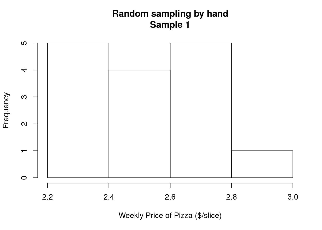
Recall from above that the mean of the entire population was 2.5660256. The mean in this first sample was 2.5186667 which is different from the population by $0.047. Does that mean our sample was “wrong”?
Of course not – but it does mean that it wasn’t “right” either. Every time we draw a sample, the exact mean will flucuate a little bit. However, we expect that, most of the time, it will land fairly close to the population mean.
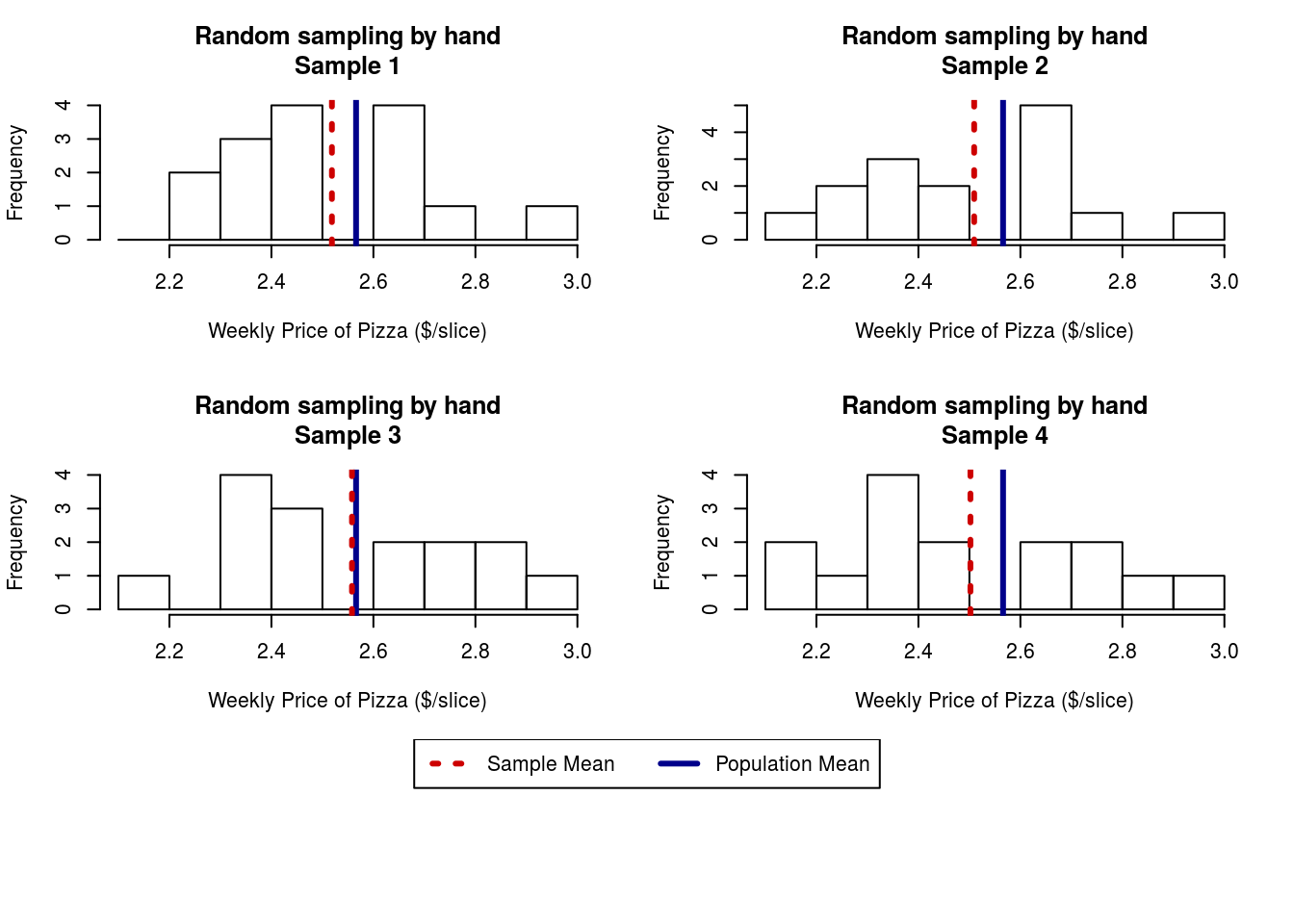
Let’s look at all 4 samples we took in class. Note that I have added a line for both the population and sample means.
10.4 Sampling in R
Now, instead of manually drawing and calculating, let’s try doing it in the computer. We will start by roughly replicating what we did by hand in class. We will draw a sample, then cacluclate the mean from it.
The function sample() draws a sample from a vector (DEN.Price from the pizza data, below) of the size (number of values) that you give in the size = argument. Here, we will use 20, which is similar to a class size.
# Draw a random sample
tempPrice <- sample(pizza$DEN.Price,
                    size = 20)
We can then look at the sample in several different ways.
# Print the values
tempPrice
## [1] 2.52 2.56 2.56 2.54 2.56 2.72 2.50 2.68 2.85 2.62 2.68 2.31 2.73 2.46
## [15] 2.64 2.54 2.70 2.36 2.48 2.43# Calculate the mean
mean(tempPrice)## [1] 2.572# Visual display of the distribution
hist(tempPrice)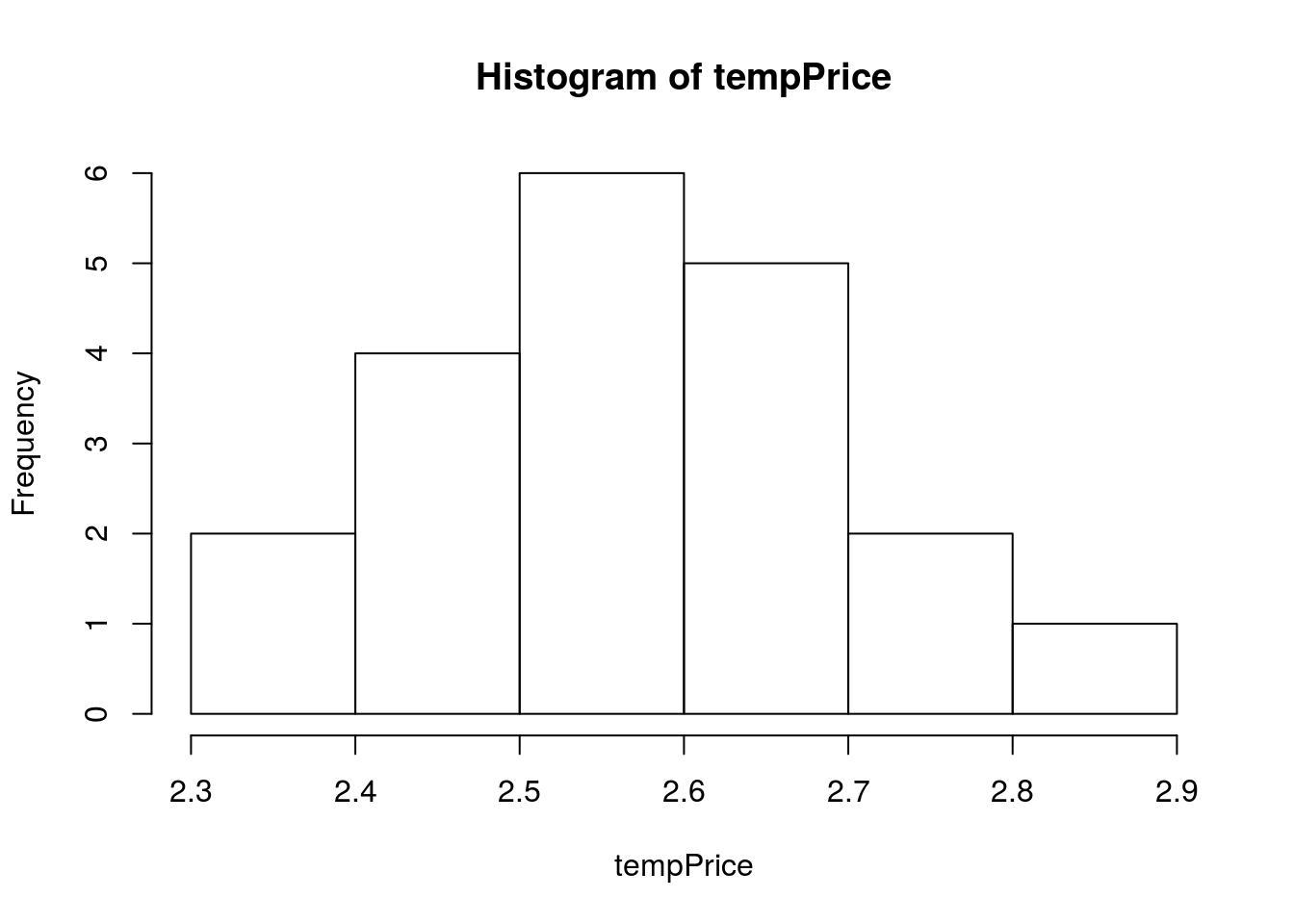
We can then compare these to the population parameters (which we know because we have access to the whole population).
# Display the true population values
mean(pizza$DEN.Price)
## [1] 2.566026hist(pizza$DEN.Price)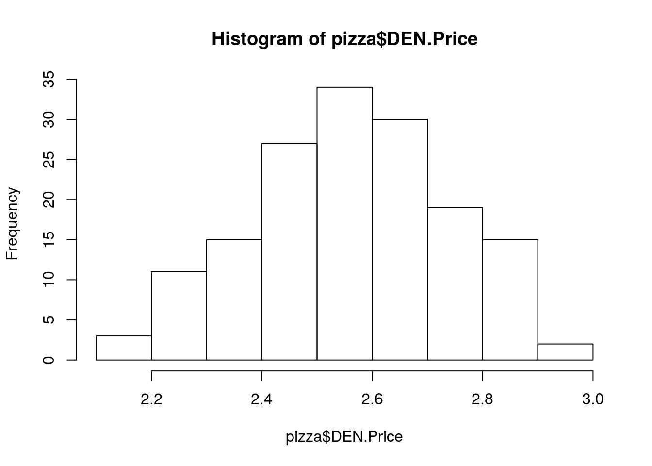
Now, go back and re-run the sample() line and the summary() of it’s outputs a few times. Notice that the output is different because the random sample selected a differnt set each time.
10.5 Repeated sampling using loops
Now, what if we want to see how “wrong” our mean tends to be? Instead of just relying on manually re-running the sample, let’s try making R do it for us. Here, we introduce the concept of a “loop” for the first time. It is just a formal way of telling the computer: “Do this {stuff} a bunch of times.”
This is an example of a for loop it travels through the loop once for each value you assign it. Here, we are using i for “index” and assigning it numeric values.
# Example Loop
for(i in c(1,2,3)){
  print(i)
}
## [1] 1
## [1] 2
## [1] 3The first argument to for() is what will be set in the loop. The part after in tells it what to set i as: here we are saying to use the values 1, 2, and 3. The loop then contains everything betewen the curly brackets “{ }”. We can put anything we want in there. Here is another example.
for(i in c(1,2,3)){
  # Comments are still ignored
  # but tell us that this will print the value of "i"
  # in each loop
  print(i)

  # This will multiply i by 3 and print the result
  print(i * 3)
}
## [1] 1
## [1] 3
## [1] 2
## [1] 6
## [1] 3
## [1] 9We can also save things in loops. Always remember to “initialize” or create the variable first, so that R knows where to put the result. If you ever get an error that reads something like: Error in myResult[i] <- i * 3 : object 'myResult' not found in a loop, the most likely culprit is that you forgot to initialize the variable (or mistyped it in one place). Here is an example of loop where we save something.
# Create an empty numberic value
myResult <- numeric()

# Run a loop and save a value
for(i in c(1,2,3)){
  # save the result in the "ith" position, hence index
  myResult[i] <- i * 3
}

# show what we saved
myResult
## [1] 3 6 9Now, we can use that to save the means of many samples. Note that I am replacing the c(1,2,3) with 1:3, which is just a short hand for: “give me every digit from 1 to 3.”
# Create an empty numberic value
myMeans <- numeric()

# Run a loop of the sample and save the mean
for(i in 1:3){
  # Copy the sampling from above
  tempPrice <- sample(pizza$DEN.Price,
                      size = 20)

  # save the mean in the "ith" position, hence index
  myMeans[i] <- mean(tempPrice)
}

# diplay results
myMeans
## [1] 2.6045 2.5420 2.6235Up until now, we could have done all of this by hand. The real advantage (and advantage of R over other tools) is that we can easily do this 1000 times (or any large number we want). Simply copy the above and change 3 to 1000 (or some large arbitrary number).
# Create an empty numberic value
myMeans <- numeric()

# Run a loop of the sample and save the mean
for(i in 1:1000){
  # Copy the sampling from above
  tempPrice <- sample(pizza$DEN.Price,
                      size = 20)

  # save the mean in the "ith" position, hence index
  myMeans[i] <- mean(tempPrice)
}
R has just calculated the means of 1000 random samples! Now, let’s take a look at those means. Note that we are no longer plotting the sampled values, but are instead plotting the means of each of the samples
# plot results
hist(myMeans)
abline( v = mean(pizza$DEN.Price),
        col = "darkblue", lwd = 3)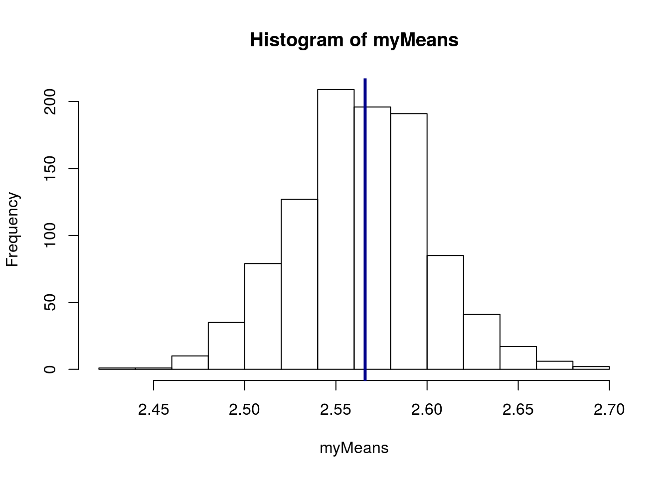
Note that the distribution is centered very close to the true population mean. We can even see how close it is:
# Calculate the mean mean:
mean(myMeans)
## [1] 2.564252# Compare to actual mean of:
mean(pizza$DEN.Price)## [1] 2.566026The other thing to note is that the distribution is much narrower, we don’t get mean values nearly as low as the cheapest week ($2.11) or as high as the most expensive week ($2.99). That is because the mean is going to minimize those extreme swings.
Below, and in more detail next lesson, we will begin to explore the details of these distributions.
10.5.1 Try it out
Take 1000 samples of the AGE of all MLB players from the mlb data. (the population). Plot the means of your samples, and explain how it differs from a plot of the population.
10.6 Sample size change
What happens if, instead of taking 20 values, we take a sample of 40 values?
# Create an empty numberic value
myMeansForty <- numeric()

# Run a loop of the sample and save the mean
for(i in 1:1000){
  # Copy the sampling from above
  # Change the "size" to 40, to take 40 samples, instead of 20
  tempPrice <- sample(pizza$DEN.Price,
                      size = 40)

  # save the mean in the "ith" position, hence index
  myMeansForty[i] <- mean(tempPrice)
}

# plot results
hist(myMeansForty)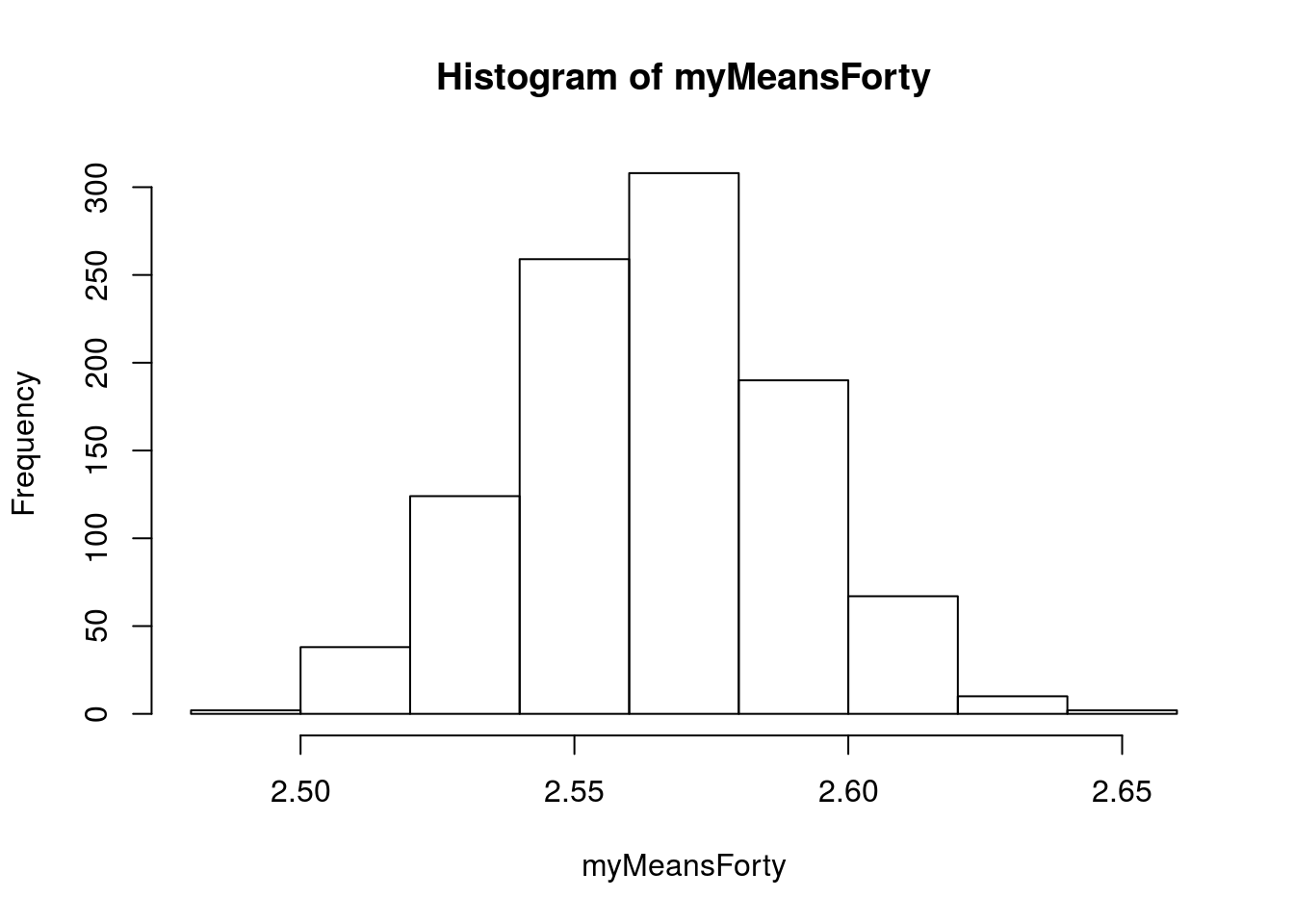
# Numeric summary
mean(myMeansForty)
## [1] 2.565133How does this distribution compare to when we only took a sample of 20 values? Let’s look. Note that I am adding the population mean to each plot, just so we have a reference.
# Change the par(mfrow) to make one plot above another
# Note also that I am setting the x limit to the same
#   range for each plot to capture the top and bottom
par(mfrow=c(2,1))

# plot the set from sample size == 10
hist(myMeans,      xlim = c(min(myMeans,myMeansForty),
                            max(myMeans,myMeansForty)))
# Add a vertical line for the mean
abline(v=mean(pizza$DEN.Price), col = "darkblue",lwd = 3)

# plot the set from sample size == 40
hist(myMeansForty, xlim = c(min(myMeans,myMeansForty),
                            max(myMeans,myMeansForty)))
# Add a vertical line for the mean
abline(v=mean(pizza$DEN.Price), col = "darkblue",lwd = 3)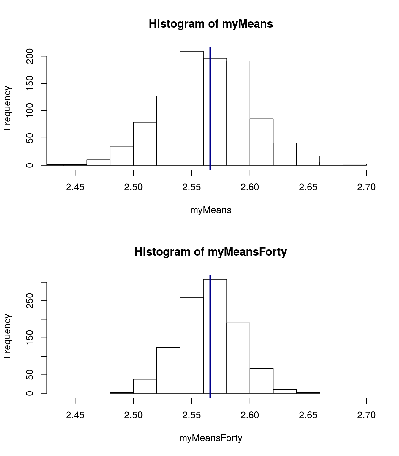
# Don't forget to set your par back
par( mfrow = c(1,1))
From the plot, which of these seems to give more accurate estimates of the population mean? Why do you think that is?
As sample size goes up, the extreme values affect the means less often. This suggests that any single mean we take from a larger sample size is likely to be closer to the true value than a mean from a smaller sample size.
10.6.1 Try it out
Change the sample size of you MLB sample a few times. What effect does it have? Try making it both larger and smaller.
10.7 Examine accuracy
We can do even better than approximating our accuracy by adding a numeric summary of how consistent we are. A measure of accuracy for samples is called the Standard Error (SE) and is just a special case of the Standard Deviation.
Because of the 95% rule, (in roughly unimodal, symmetric data, 95% of values fall within 2 sd of the mean), we can estimate that roughly 95% of our sample means will fall within 2 SE of the true population mean. This is an important point that will be discussed in more detail in the next chapter. To calculate, we use the same function we use to calculate sd’s of population and samples.
# for our samples of size 20
sd(myMeans)
## [1] 0.03730978# For our samples of size 40
sd(myMeansForty)## [1] 0.02485234Note how much smaller the SE is from the larger sample sizes. This suggests that we should have more confidence in larger samples, and supports our intuition about the differnces.
10.7.1 Try it out
Calculate the standard error of your MLB sampling distribution for at least two different sample sizes.
10.8 The importance of a random sample
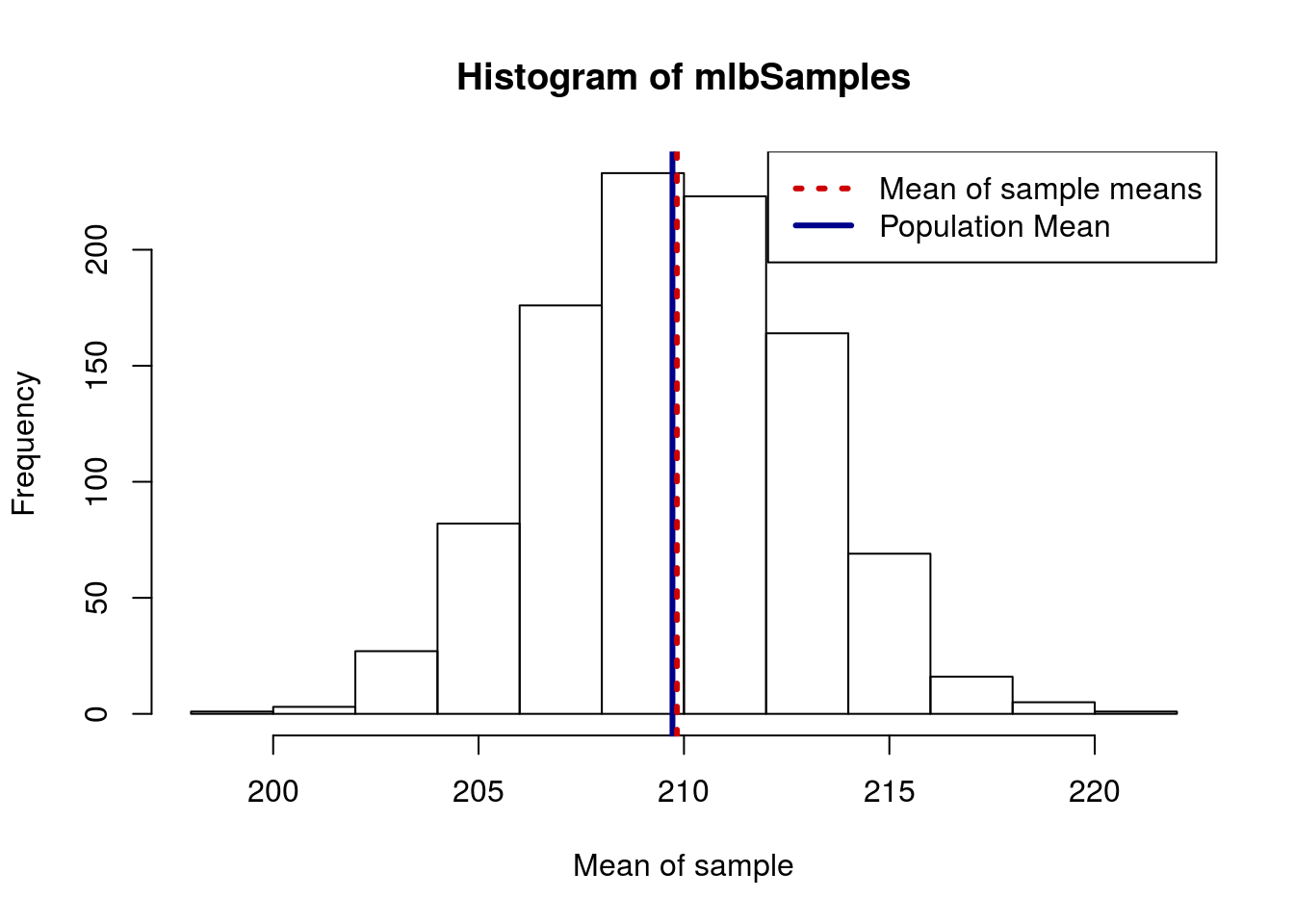
Always be careful that you are drawing a representative sample. If your sample is not representative, your estimate of the population is not likely to be accurate. For instance, compare these approaches to sampling Mlb Weights.
# See where we should be
mean(mlb$Weight)
## [1] 209.72# Generate several samples
mlbSamples <- numeric()
for(i in 1:1000){
# Copy the sampling from above
tempWeight <- sample(mlb$Weight,size = 40)
# save the mean in the "ith" position, hence index
mlbSamples[i] <- mean(tempWeight)
}
# plot results
hist(mlbSamples,
xlab = "Mean of sample")
# Add lines
abline(v = mean(mlb$Weight), col = "darkblue", lwd = 3)
abline(v = mean(mean(mlbSamples)),
col = "red3", lwd = 3, lty = 3)
# Add legend
legend("topright",
legend = c("Mean of sample means","Population Mean"),
lty = c(3,1), lwd = 3,
col = c("red3","darkblue")
)
However, what if, instead, we accidentally sample only Pitchers? Note here that, within sample, I am limiting to only those players where mlb$POS.Broad == "Pitcher".
# Generate several samples
mlbBiasedSamples <- numeric()
for(i in 1:1000){
  # Copy the sampling from above
  tempWeight <- sample(mlb$Weight[mlb$POS.Broad == "Pitcher"],
                       size = 40)
  # save the mean in the "ith" position, hence index
  mlbBiasedSamples[i] <- mean(tempWeight)
}

# plot results
hist(mlbBiasedSamples,
     xlab = "Mean of sample")

# Add lines to show means
abline(v = mean(mlb$Weight), col = "darkblue", lwd = 3)
abline(v = mean(mean(mlbBiasedSamples)),
       col = "red3", lwd = 3, lty = 3)

# Add a legend
legend("topright",
       legend = c("Mean of sample means","Population Mean"),
       lty = c(3,1), lwd = 3,
       col = c("red3","darkblue")
       )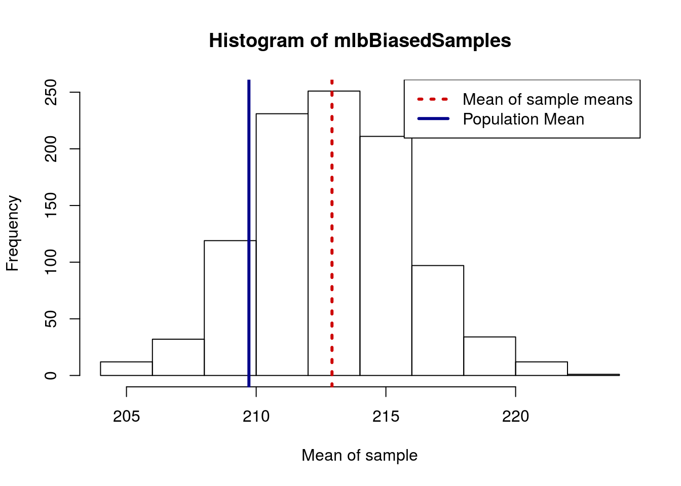
While, in R, this seems like it would be difficult to “accidentally” do, in the real world, such errors are rather common. Imagine, if you will, that we wanted to sample player weights as early as we could, so we went to Spring Training the day that it opened for each team. Do you know who the first players are to report?
It turns out that pitchers and catchers are the first ones to camp. This would make it relatively easy to mistakenly get the wrong picture of MLB player weights if we weren’t careful about our samples.
10.8.1 Try it out
From the mlb data, repeatedly take samples of the Weight of players size 10 (that is, sample the weight of 10 players each time) from only the Pittsburgh Pirates. Compare that to the true population value.
This would be the equivalent of going to just the Pirates, collecting a small sample, then trying to say something about all MLB players. Does it appear that this is a reasonable sampling method?