13.1 Load today’s data

Start by loading today’s data. If you need to download the data, you can do so from these links, Save each to your data directory, and you should be set.

• NFLcombineData.csv
  • Data on the Height, Weight, and position type of all 4299 players that participated in the NFL combine during the collection period
• hotdogs.csv
  • Data on nutritional information for various types of hotdogs
• Roller_coasters.csv
  • Data on Roller coasters

# Set working directory
# Note: copy the path from your old script to match your directories
setwd("~/path/to/class/scripts")

# Load data
nflCombine    <- read.csv("../data/NFLcombineData.csv")
rollerCoaster <- read.csv("../data/Roller_coasters.csv")
hotdogs       <- read.csv("../data/hotdogs.csv")

13.2 The limitations of the SE estimate

In the previous chapter, We have glossed over a problem: how can we calculate a confidence interval if we want to be something other than 95% sure? How can we get a 90% confidence interval? Or 99% or 42% or 90.0461%?

This chapter will introduce an alternative way to empirically estimate our confidence interval: directly calclulating percentiles. Instead of estimating where the data are likely to fall, we will calculate it directly from our bootstrap samples.

This method is broadly applicable and gives us much more flexibility (and accuracy). We will start by applying it to bootstraps conducted in the previous chapter, but will extend it to show the application of bootstrapping to two new populations as well.

Recall from yesterday that we collected 15 beads as a sample to estimate the proportion of beads that were red in the population.

# Enter the data from the class sample
classBeadSample <- rep(c("red", "white"),
                       c(  10 ,   5   ) )

propRedSample <- mean(classBeadSample == "red")
propRedSample

## [1] 0.6666667

We then bootstrapped a distribution to estimate the standard error (copied from the previous chapter).

# Initialize our variable (we can use the same one we used above)
inClassBootStats <- numeric()

# Loop an arbitrarily large number of times
# More will give you a more accurate and consistent distribution
for(i in 1:8793){
  # collect a sample
  tempBootSample <- sample(classBeadSample,
                           size = length(classBeadSample),
                           replace =  TRUE) # NOTE: we need this line
    
  # Store the value in the first slot
  inClassBootStats[i] <- mean(tempBootSample == "red")
}

We can then look at our distribution and mark our 95% confidence interval based on the standard deviation:

hist(inClassBootStats,
     xlab = "Sample Proportion Red")

abline(v = mean(inClassBootStats) + c(-2,2)*sd(inClassBootStats),
       col = "green3", lwd = 3, lty = 2)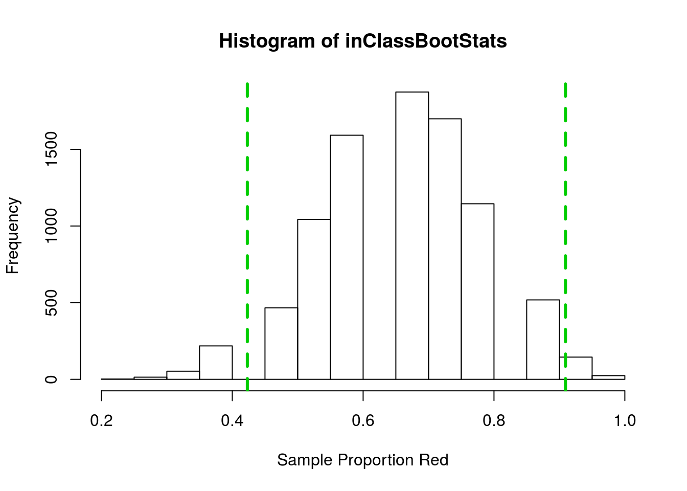

This gave a 95% confidence interval between 0.42 and 0.91. But what if we only wanted to be 90% sure we had the true mean? We could then make the interval a little smaller, but how much smaller? What if instead we wanted to be 99% confident? We would then have to make the interval wider, but how much wider?

13.3 Directly calculating confidence interval

Instead, let’s just compute where 95% of the data lie directly. You can probably eyeball this from the histogram, but let’s make it explicit.

One note here before we go further. These data are not ideal for this because the values are so discrete – with only 15 beads, there are only 16 possible values of the sample proportion; however, it is still good enough for this illustration, and good enough to make statements about the population.

Recall from earlier classes that we can calculate the quartiles easily with the function summary() as such:

summary(inClassBootStats)

##    Min. 1st Qu.  Median    Mean 3rd Qu.    Max. 
##  0.2000  0.6000  0.6667  0.6662  0.7333  1.0000

Because half of the data fall between the first and third quartiles, we could say that our 50% confidence interval is between 0.6 and 0.7333.

But, we are rarely interested in a 50% confidence interval. Instead, we want to be able to find the middle any percentof the data. To do this, we need to be able to calculate any percentile we are interested in. A percentile is just the proportion of data at and below a certain point. It is commonly used in standardized tests. For example, on the ACT a composite score of 34 is as good or better than 99% of the people that took the test, making it the 99th percentile. A score of 30 is at the 90th percentile, meaning only 10% of students scored better than that. At the other end, a composite score of 14 is only as good or better than 12% of students, making it the 12th percentile.

To calculate the 95% confidence interval, we need to introduce a new function quantile(). It takes a vector (such as our bootstrap sample statistics) and calculates any percentile we ask it for. We will generally want at least a couple, and we can ask for multiples using c() to hold our values. Here is an example showing the quartiles.

quantile(inClassBootStats, c(0.25, 0.75))

##       25%       75% 
## 0.6000000 0.7333333

If we want a 95% confidence interval, we need to get the middle 95%, which means that we need to break the other 5% in half, leaving 2.5% in each tail. In R, we use proportions instead of percents, so get the values like this:

# Calculate 95% CI
quantile(inClassBootStats, c(0.025, 0.975))

##      2.5%     97.5% 
## 0.4000000 0.8666667

Which tells us that 95% of our values fall between 0.4 and 0.8666667, which is very similar to our CI calculated above using the standard error. However, now we can use this to calculate a number of different sized confidence intervals:

# Calculate 99% CI
quantile(inClassBootStats, c(0.005, 0.995))

##      0.5%     99.5% 
## 0.3333333 0.9333333

# Calculate 90% CI
quantile(inClassBootStats, c(0.05, 0.95))

##        5%       95% 
## 0.4666667 0.8666667

And here they are plotted, showing the differences in size

hist(inClassBootStats,
     xlab = "Sample Proportion Red")

# Add the various CI's
abline( v = quantile(inClassBootStats, c(0.005, 0.995)),
        col = "red3", lwd = 3, lty = 3)
abline( v = quantile(inClassBootStats, c(0.025, 0.975)),
        col = "green3", lwd = 3, lty = 3)
abline( v = quantile(inClassBootStats, c(0.05, 0.95)),
        col = "darkblue", lwd = 3, lty = 3)
legend("topleft", inset = 0.01,
       legend = c(90,95,99),
       title = "CI level",
       col = c("darkblue","green3","red3"),
       lwd = 3, lty = 3)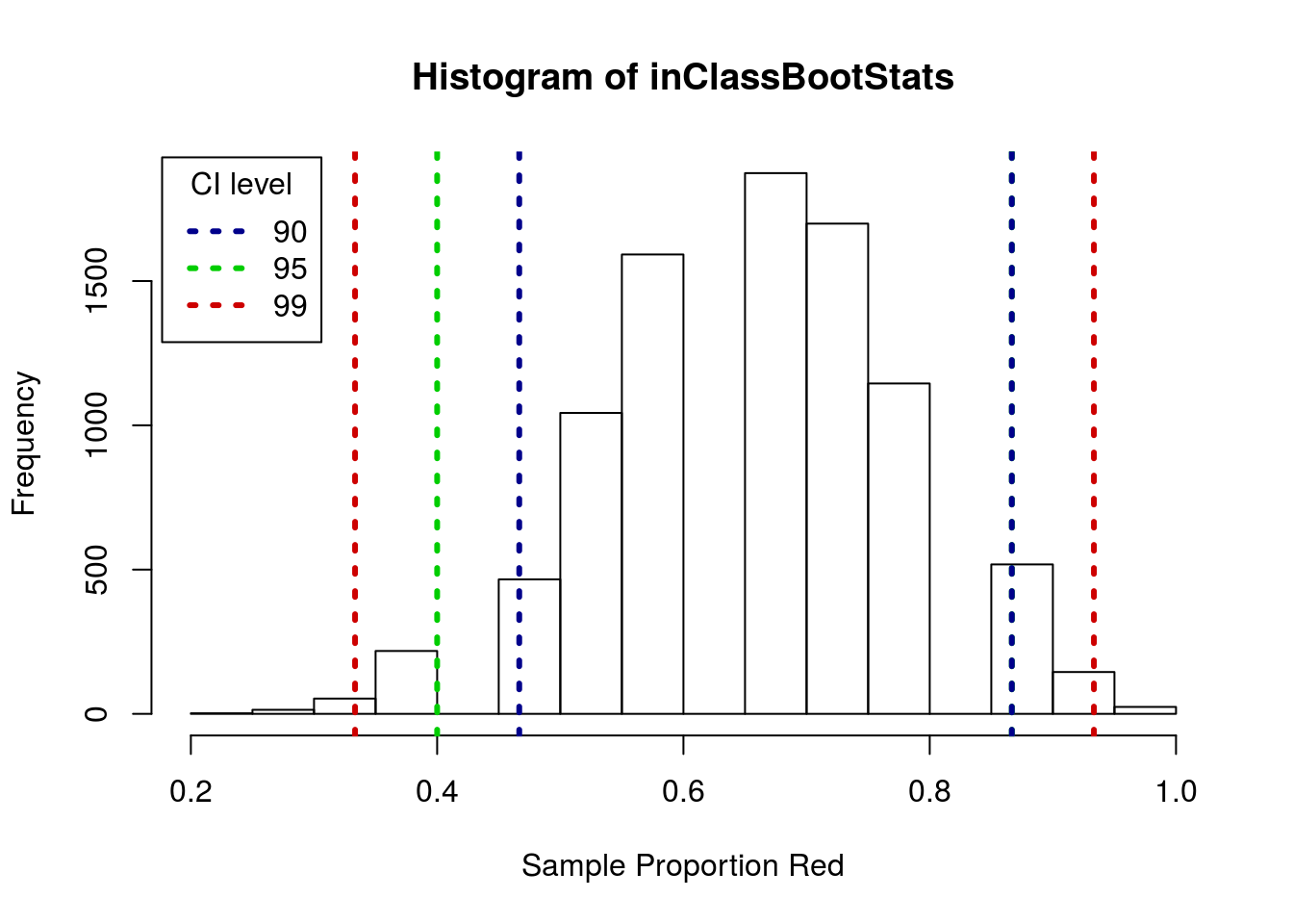

Note that, because of the discrete steps, the top of the 99% and 95% CI’s happen to fall at the same point. In larger samples, or samples calculating thigns other than proportions, that is much less likely to happen.

13.4 Bootstrap for a mean

With this new tool in hand, let’s see how it applies to something like a mean. Here, we treat the Drop column of rollerCoaster as a sample representative of all roller coasters. To start, let’s look at the distribution:

# Plot it, see how it makes us feel
hist(rollerCoaster$Drop,
     main = "Roller Coaster Heights",
     xlab = "Max Drop (Feet)")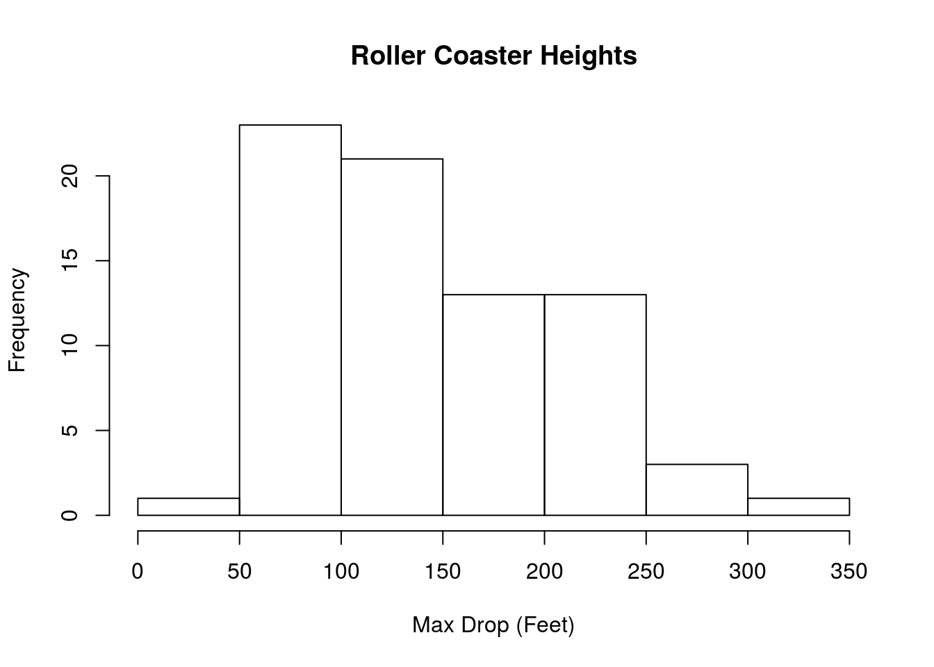

The center appears to be somwhere around 150 feet tall. But, we can (and should) calculate it directly:

mean(rollerCoaster$Drop)

## [1] 145.7549

Does this mean that the average height of all roller coasters is exactly 145.7549333? Of course not. Does it mean that our best guess at the average height is about 146? Yep. Without any other information, we would say that we think roller coasters are probably “about” 146 feet tall on average.

But … what do we mean by “about,” and how sure are we? This is where confidence intervals and bootstrapping come into play. Because we don’t have the whole population, we need to work from this sample to estimate the heights. So, we set up a bootstrap sample like we did before.

# Initialize vector
coasterBoot <- numeric()

# Loop through the sample
for(i in 1:12489){
  # take a bootstrap sample
  tempCoasterboot <- sample(rollerCoaster$Drop,
                            size = nrow(rollerCoaster),
                            replace = TRUE)
  # Save the mean
  coasterBoot[i] <- mean(tempCoasterboot)
}

Now, instead of calculating the standard error, let’s empirically determine where the values fall to get a 90% confidence interval. Use quantile() again, remembering that we want to split that “remaining” 10% into each tail.

# Calculate 90% CI
quantile(coasterBoot, c(0.05, 0.95))

##       5%      95% 
## 134.7218 156.9069

Tells us that our 90% confidence interval ranges from 134.72176 feet to 156.9069333 feet, meaning that we are 90% confident the true mean falls in that range.

But, what if we needed to be really, really sure? We could calculate a 99% interval

# 99% interval
quantile(coasterBoot, c(0.005, 0.995))

##     0.5%    99.5% 
## 128.5898 163.1819

If we had to make sure that our confidence interval definitely contained the true mean, we could just say that the mean is probably somewhere between 0 feet and 1,000 miles. But, that is not particularly useful. In practice, we must tradeoff the desire to capture the true mean within the interval with the desire to make a precise estimate.

Finally, we can (and should) plot a histogram of our sample with our confidence interval marked. That will help us spot any problems that may have arisen.

# Plot the bootstrap with 90% CI
hist(coasterBoot,
     xlab = "Sample mean Drop (Feet)")
abline(v = quantile(coasterBoot, c(0.05, 0.95)),
       lwd = 3, lty = 3, col = "magenta")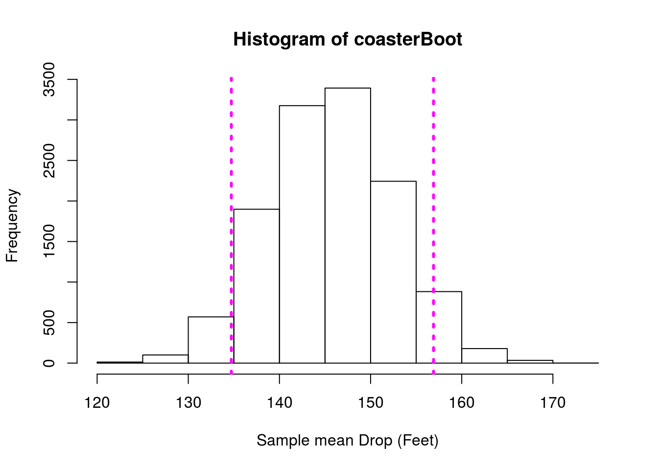

Here, we don’t know the true population parameter, and so we have no way of “checking” our answer. That is how statistics works. We have been using (and will continue to see examples of) full populations to illustrate these concepts. However, that is not what you will be encountering once you leave this class and start analyzing your own data.

13.5 Bootstap estimate of a difference

Returning the NFL data, what if, from a sample of the players that attended the combine, we wanted to estimate the difference in weight between linemen and skill players? Recall that we can use sampling and bootstrapping on just about any sample statistic we want, then let’s give it a try.

First, let’s collect a sample of each type of player. The number we collect is arbitrary, but should be large enough that we think it will give a good estimate.

# Set seed for consistent results on re-runs
set.seed(16652)

# Collect a sample from each
lineSample  <- sample(nflCombine$Weight[nflCombine$positionType == "line"],
                      size = 38)
skillSample <- sample(nflCombine$Weight[nflCombine$positionType == "skill"],
                      size = 43)

Let’s visualize the sample, which is always a good idea.

boxplot(skillSample,lineSample,
        names = c("skill","line"),
        xlab = "Position type",
        ylab = "Weight (lbs)")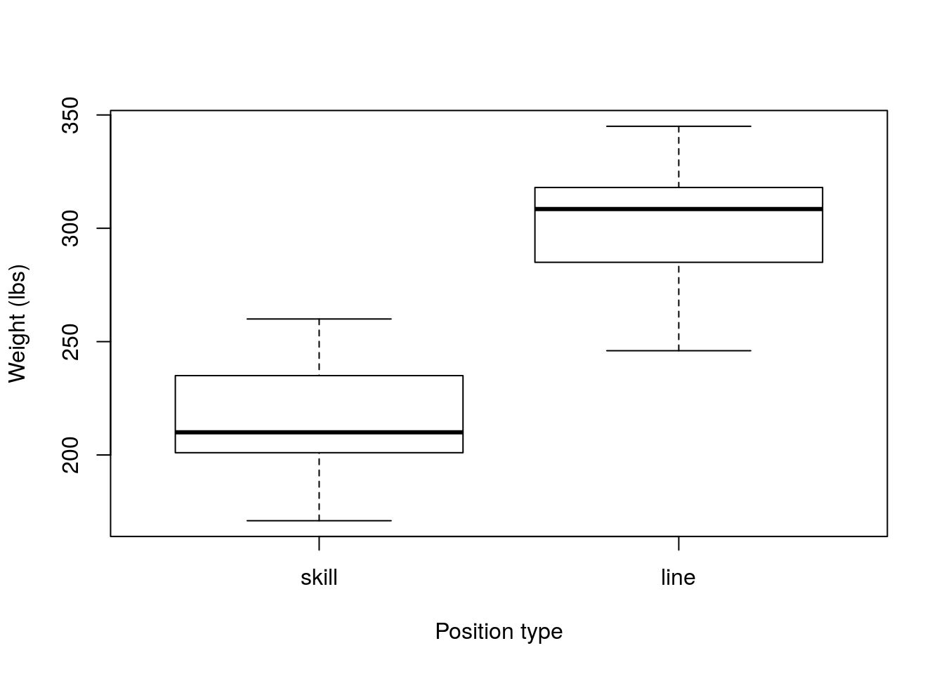

Now, we should calculate our point estimate for the population (the value of the sample statistic).

mean(lineSample) - mean(skillSample)

## [1] 87.20624

This sample suggests that linemen weigh 87.21 lbs more than skill postition players. However, we would like to know how much trust to put in our sample, so, let bootstrap. As before, we need to make sure that each sample is the same size as it’s original value (R automatically does this, so we won’t be setting the size = argument here), and that we sample with replacement. However, we now need to construct two new samples and our test statistic is the difference between them.

First, let’s try doing a few boot strap samples by hand, so that we can see them.

set.seed(47403)

# initialize a variable to hold differences
weightDiff <- numeric()

# Construct bootstrap samples for each position type
tempLine  <- sample(lineSample, replace = TRUE)
tempSkill <- sample(skillSample, replace = TRUE)

# Store the difference in the means
weightDiff[1] <- mean(tempLine) - mean(tempSkill)

# Show the value
weightDiff

## [1] 98.85741

This has stored the difference of one bootstrap sample. Next, lets add a few more.

# Construct a NEW bootstrap samples for each position type
tempLine  <- sample(lineSample, replace = TRUE)
tempSkill <- sample(skillSample, replace = TRUE)

# Store the difference in the means
weightDiff[2] <- mean(tempLine) - mean(tempSkill)


# Construct a NEW bootstrap samples for each position type
tempLine  <- sample(lineSample, replace = TRUE)
tempSkill <- sample(skillSample, replace = TRUE)

# Store the difference in the means
weightDiff[3] <- mean(tempLine) - mean(tempSkill)


# Show the value
weightDiff

## [1] 98.85741 92.40514 89.81334

Now, we could copy that a thousand times, but you may have noticed that the only thing changing which index in weightDiff we are storing the difference in. Instead, we can copy those exact lines of code into a for() loop, change the number (e.g. 1, 2, or 3 above) to “i”, and run it as many times as we want. This loop is equivalent to copying the above lines 10,458 times (but is a lot easier). In reality, we often want to try 1 run through a loop, similar to what we did above, but don’t (usually) need to do more than that.

# Set seed for consistent results on re-runs
set.seed(47403)

# initialize the variable
weightDiff <- numeric()

# loop an arbitrarily large number of times
for(i in 1:10548){
  # Construct bootstrap samples for each position type
  tempLine  <- sample(lineSample, replace = TRUE)
  tempSkill <- sample(skillSample, replace = TRUE)
  
  # Store the difference in the means
  weightDiff[i] <- mean(tempLine) - mean(tempSkill)
}

Now, let’s visualize our result and construct a 95% confidence interval.

# Look at the distribution of the bootstrap sample stats
hist(weightDiff)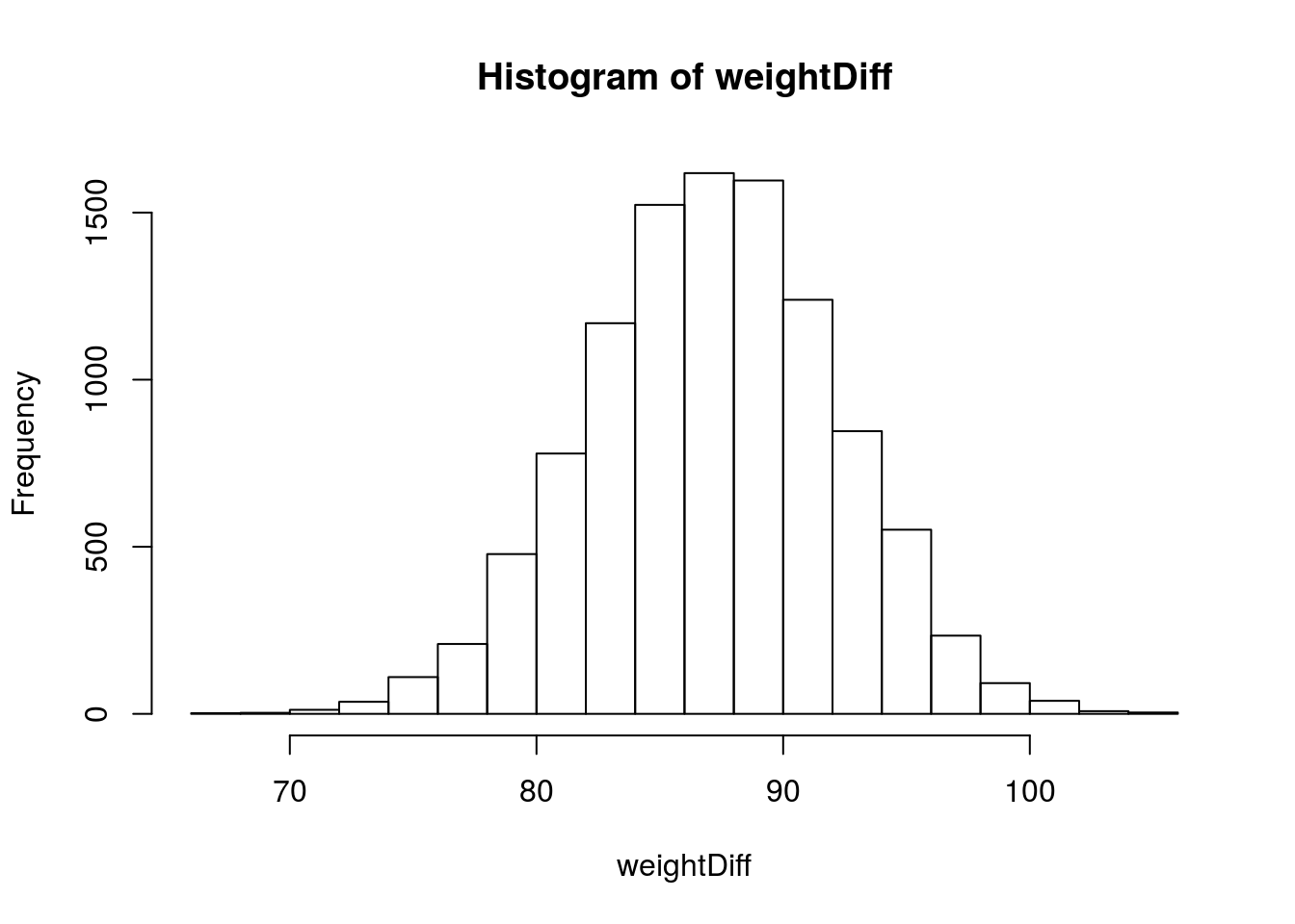

# calculate our 95% interval
quantile(weightDiff, c(0.025, 0.975))

##     2.5%    97.5% 
## 77.15711 96.80598

Which says that we are 95% certain that the true difference in weight between linemen and skill players is somewhere between 77.16 lbs and 96.81 lbs, with our point estimate still at 87.21. Importantly, this tells us that linemen are almost certainly heavier than skill position players, even if we aren’t quite sure by how much. We will begin to explore this idea in more depth soon.

Looking at our true population difference we see that this range is a reasonable one.

mean(nflCombine$Weight[nflCombine$positionType == "line"]) - 
  mean(nflCombine$Weight[nflCombine$positionType == "skill"])

## [1] 82.89531

13.6 A final example with correlation

Finally, I just want to include an example where we estimate a correlation. In previous chapters, we have used the rollerCoaster data to calculate the correlation between Drop and Speed. However, there are more roller coasters in the world than just these 75. How certain are we that they represent the correlation for all roller coasters? To estimate this, we will treat these 75 roller coasters as a sample, and all roller coasters in the world as the population.

First, let’s plot our data and calculate the correlation for this sample.

# Plot the data
plot(Speed ~ Drop, data = rollerCoaster)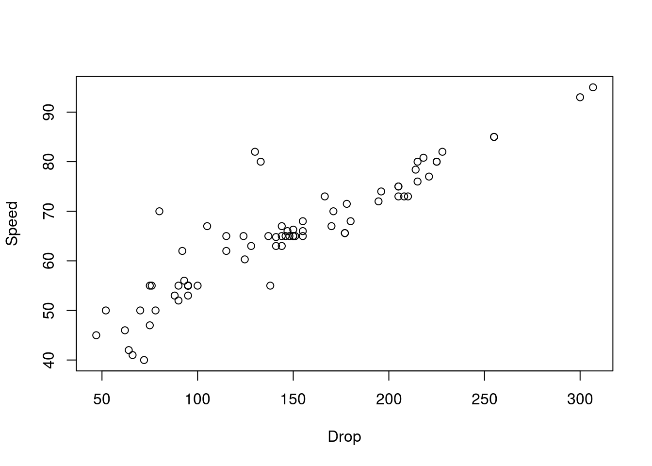

# Calculate the correlation
cor(rollerCoaster$Speed, rollerCoaster$Drop)

## [1] 0.9096954

Next, let’s take many bootstrap samples of the data. As with the comparison of weight, we need to collect two samples, however, these data (because we are interested in correlations) are paired. So, when we sample, we need to make sure we take them in the same order. To do this, instead of sampling from the values themselves, we will sample an index, which will tell us which value to take.

An example:

# Sample an index
mySample <- sample(1:5, replace = TRUE)

# look at those rows of the coaster data
rollerCoaster[mySample,]

##                   Name Speed Drop
## 3               Titan     85  255
## 5          Xcelerator     82  130
## 1    Millennium Force     93  300
## 1.1  Millennium Force     93  300
## 4   Phantom's Revenge     82  228

# look each Speed and drop
rollerCoaster$Speed[mySample]

## [1] 85 82 93 93 82

rollerCoaster$Drop[mySample]

## [1] 255 130 300 300 228

Note a few things here, first, in this sample we got a duplicate of one our rows, because we are sampling with replacement. Second, whether we use the mySample variable in the data frame, or calling the vector directly, we get the same values, and they are still paired (you can see this from the names in the data.frame output). Finally, we only sampled from 1 to 5 for illustrative purposes, but for the full set, we will sample from 1 to the number of rows in the data.frame. (we could also use the length of one of the column vectors, this is just another solution, both give the same value).

# Initialize vector
coasterBoot <- numeric()

# Loop through many times
for(i in 1:12489){
  # Sample from your indices
  mySample <- sample(1:nrow(rollerCoaster),replace = TRUE)
  
  # calculate the correlation
  # note, we could save these each as a vector first
  # but we don't need to 
  coasterBoot[i] <- cor(rollerCoaster$Speed[mySample],
                        rollerCoaster$Drop[mySample])
}

Now, we again visualize and calculate a confidence interval.

# Plot the result
hist(coasterBoot, xlab = "Bootstrap sample correlation")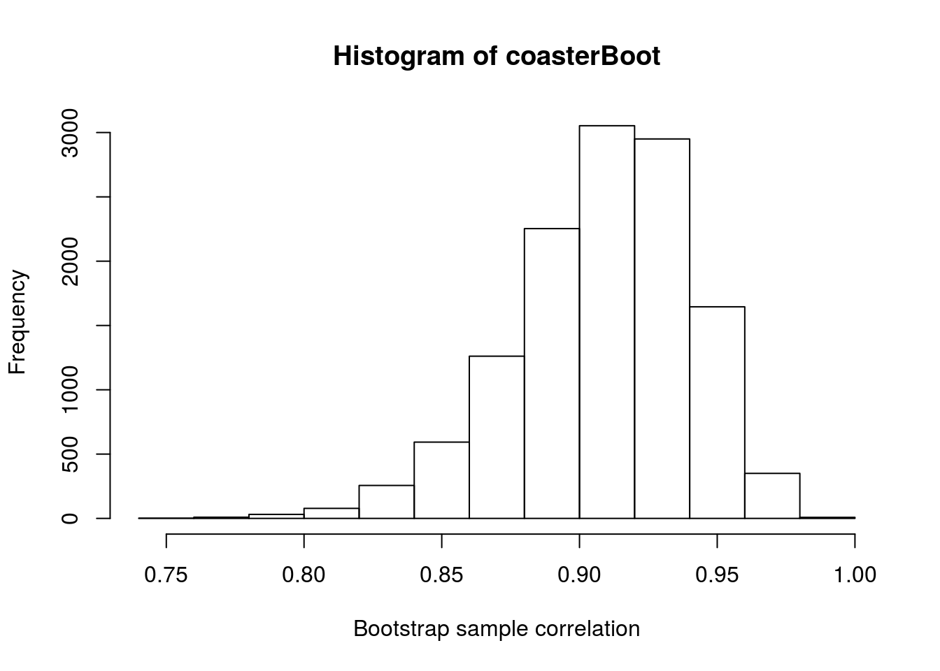

# Calculate the 95% confidence interval
quantile(coasterBoot, c(0.025, 0.975))

##      2.5%     97.5% 
## 0.8366620 0.9611161

From this, our population point estimate is still 0.91, and we have 95% confidence that our true population correlation is somewhere between 0.837 and 0.961.