21.1 Load today’s data

There is no data to load for this chapter.

21.2 Testing a null hypothesis

In the last lesson we introduced a short cut to estimate the standard error of the sampling distribution for a proportion:

\[ SE = \sqrt{\frac{p \times (1-p)}{n}} \]

There we also saw it applied to bootstrap distributions to estimate confidence intervals. We have also been using re-sampling to construct null distributions, and may want to use the short cut for those as well.

Here, our job is even a bit easier: our null value (mean for the normal model) is just whatever the null hypothesis says it should be, and the SE is just calculated from that. We can then figure out how likely (or unlikely) our data (or more extreme data) would be if the null hypothesis were true. For n, we just use whatever our sample size is.

For example, let’s say that, we expect stop lights should be green one-third of time because there are three colors. Using that as our null, we can build the sampling distribution for the proportion if we record the color of the light at 50 intersections. Let’s start by sampling many times.

Note that here, I am using prob = in sample() to control how likely R is to sample each value. In the past we have generally created a vector with the proportions we desire (e.g. one “green” and two “notGreen”), that can get a bit cumbersome for more complicated values. Instead, we can just create a vector with each thing once, then tell R to sample each of them at a particular rate. Each entry after prob = matches to the entries that are being sampled, and gives the probability for that value.

# Set null Prop
nullProp <- 1/3

# Set our n
n <- 50

# initialize the variable
propGreenNull <- numeric()

# Loop to sample
for(i in 1:15678){
  tempSample <- sample(c("green","notGreen"),
                       size = n,
                       replace = TRUE,
                       prob = c(nullProp, 1-nullProp))
  propGreenNull[i] <- mean(tempSample  == "green")
}

# Visualize
hist(propGreenNull,
     breaks = 20,
     xlab = "Sample proportion that are green")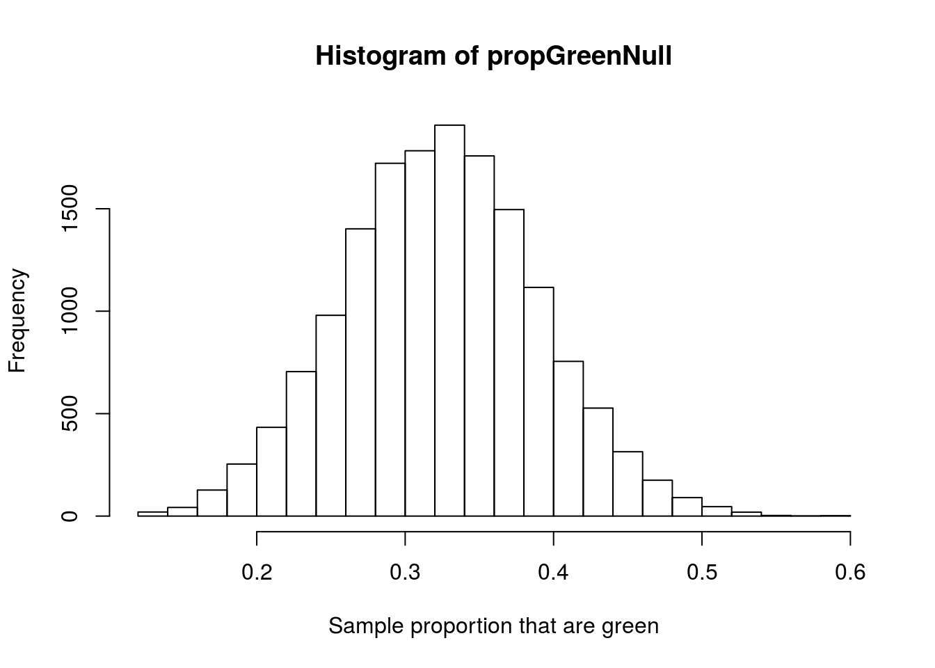

Note that I set the breaks purely for aesthetic reasons, it just seems to look nicer. This gives us, as before, a nice, normal-looking distribution. We can thus use the short cut above to estimate the standard error.:

# Set null SE
nullSE <- sqrt( ( nullProp*(1-nullProp) ) / n )
nullSE

## [1] 0.06666667

We can compare that to our observed standard error:

# Observed SE
sd(propGreenNull)

## [1] 0.06587311

and see that they are very similar. Now, just as before, we can calculate the area under the curve that is as ,or more, extreme than some observed data. Imagine that you had recorded the last 50 lights you had driven through, and found that only 10 of them were green. We can test to see how likely you were to hit 10 (or fewer) greens in those 50 lights using the function pnorm().

# Set our data (especially useful when working from csv files)
propGreenHit <- 10/50

# Calculate more extreme values
pnorm(propGreenHit,
      mean = nullProp,
      sd   = nullSE)

## [1] 0.02275013

This tells us that only 2.28% of the time will someone hit 10 or fewer greens in 50 lights. Recall that this is only a one-tailed test. Because the distribution is symmetric, we can double it to get the total area that is more extreme than our observed data:

# Calculate two-tailed more extreme values
2* pnorm(propGreenHit,
         mean = nullProp,
         sd   = nullSE)

## [1] 0.04550026

21.3 Margin of error and picking sample size

Let’s revisit our, perhaps naive, assumption from above. Nothing about there being three options (e.g., Green, Yellow, and Red) implies that all of the values are equally likely. Further, from our experience, we know that different lights have different proportions of time in each color. As a simple case, imagine the intersection where a a small street crosses a major highway. We expect that the light will be green most of the time on the highway, and not very often for the small street.

However, we have the tools to be more specific than “not very often.” We can, instead, construct a confidence interval. To do that, we estimate the standard error, then use qnorm() (see the previous chapter for more information). Let’s use our 10 in 50 lights as an example.

# Set proportion of greens hit and number of lights observed
propGreenHit <- 10/50
n <- 50

# estimate SE
seGreen <- sqrt( propGreenHit * (1 - propGreenHit) / n)

# Calculate CI
qnorm(c(0.025, 0.975),
      mean = propGreenHit,
      sd   = seGreen)

## [1] 0.08912769 0.31087231

This means that, given our sample, we are 95% confident that the true proportion of lights that are green is between 0.089 and 0.311. That range seems rather large. What if we really need to know this value in order to plan our fastest getaway route route to school to learn?

We have seen that increasing sample size decreases the width of our distributions, so we could just go back and sample some more. But … how much more?

The answer depends on how precise we want to be. The term for this precision is usually “Margin of error,” which we have seen before. The margin of error is the distance from our point estimate to either end of the distribution. Here, we can calculate it by subtracting the observed from the top end of the range:

# Calclulate margin of error
qnorm(c(0.975),
      mean = propGreenHit,
      sd   = seGreen) - propGreenHit

## [1] 0.1108723

This tells us what we might already have realized, that our range includes ± 0.111 on either side of our observed value. You probably also noticed that propGreenHit is in that formula twice. That is because the normal is centered at the mean, so we could just leave the mean out and get the same thing:

# Calclulate margin of error
qnorm(0.975,
      sd   = seGreen)

## [1] 0.1108723

Now all we are setting is the standard deviation. Because the width of all normal distributions is just affected by the standard deviation, we can go one step further. We can calculate the z-score theshold (which recall has a sd of 1) and multiply it by our standard error (which just gives the “step” size for the normal):

# Calclulate margin of error
qnorm(0.975) * seGreen

## [1] 0.1108723

All we have done here is derive why the z* (z critical) value method works. Note that the qnorm(0.975) is going to give you the exact same value, no matter what standard error you mutliply it by. In math notation, that looks like this:

\[ ME = z^* \times SE \]

Now, this gives us some additional abilities. Because we know that the standard error is affected by the sample size, we can solve for n in order to set any margin of error we want

\[ ME = z^* \times \sqrt{\frac{p \times (1-p)}{n}} \]

divide by z* and re-write the square root

\[ \frac{ME}{z^*} = \frac{\sqrt{p \times (1-p)}}{\sqrt{n}} \]

Multiply each side by \(\sqrt{n}\)

\[ \sqrt{n} \times \frac{ME}{z^*} = \sqrt{p \times (1-p)} \]

Multiply each side by \(\frac{z^*}{ME}\)

\[ \sqrt{n} = \frac{z^*}{ME} \times \sqrt{p \times (1-p)} \]

Square it all:

\[ n = \left(\frac{z^*}{ME}\right)^2 \times p \times (1-p) \]

So, for any value of p, we can calculate the n needed to get any precision of ME that we would like. So, if we think that the most likely value the proportion of time the light is green is the 0.20 we observed before, we can calculate the n need to get a margin of error of 0.03.

# Calculate needed N
(qnorm(.975) / .03)^2 * propGreenHit * (1 -propGreenHit)

## [1] 682.926

Because we want a margin of error that is no bigger than the one we asked for, we always use the next highest integer. So, if we wanted a margin of error of 0.03, we would need to observe the stop light 683 times.

In practice, researchers either use their estimate of the proportion or 0.5 for the value of p. Using 0.5 gives the largest ME, and so is the safest in terms of estimation. If we plug in 0.5 for p above, we get:

# Calculate needed N
(qnorm(.975) / .03)^2 * 0.5 * (1 - 0.5)

## [1] 1067.072

You will likely notice that the sample sizes for most polls you see on the news and in print give a margin of error of about ± 3 percentage points and have a sample size of around 1000. This is the standard in the industry in large part because the sample size goes up so dramatically to get more accurate. Imagine we instead want an ME of 0.02

# Calculate needed N
(qnorm(.975) / .02)^2 * 0.5 * (1 - 0.5)

## [1] 2400.912

We need to more than double the sample size. To get to an ME of 0.01 is even more difficult:

# Calculate needed N
(qnorm(.975) / .01)^2 * 0.5 * (1 - 0.5)

## [1] 9603.647

There are diminishing returns in increasing sample size, and the cost of collecting a bigger sample is often not worth the marginal gain in accuracy.

21.4 Assumptions

These shortcuts come with a large number of assumptions, all of which are true enough for most applications. However, we do need to be a bit wary when applying them. Always check that your data are actually amenable to the normal model. As we saw from the Central Limit Theorem, that usually means that the sample size is big enough.

For proportions, “big enough” sample size means that for the proportion we are dealing with, we expect at least 10 values in each category. We can see why this is if we plot the curve we generate for a sample of size 20 with a population proportion of 0.1.

popProp <- 0.1
n <- 20

# Calculate se
se <- sqrt( ( popProp*(1-popProp) ) / n )

# Draw the curve
curve(dnorm(x, mean = popProp, sd = se),
      from = -0.2,
      to = 0.4)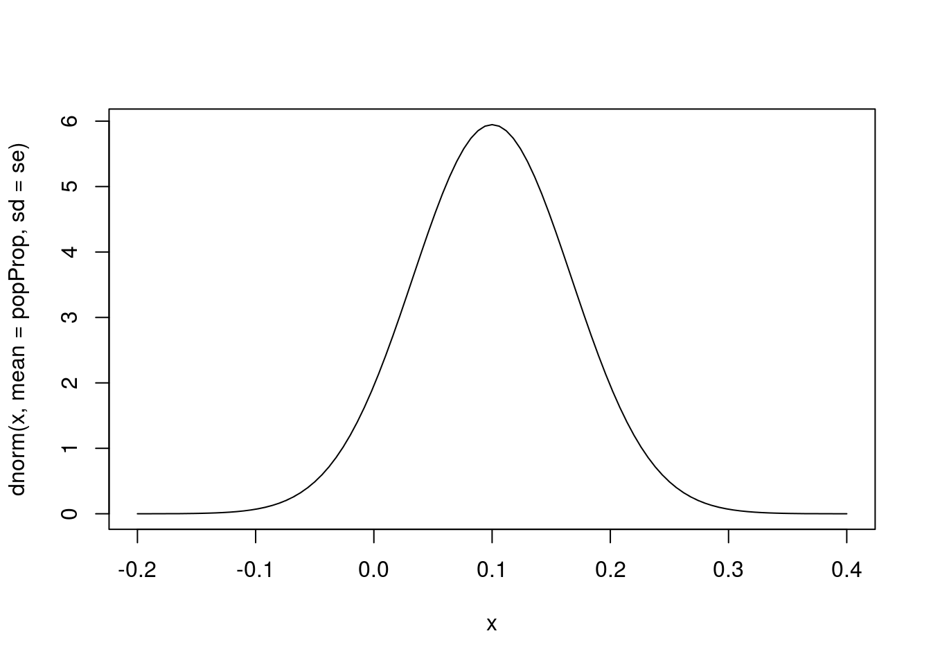

Notice that a good portion of the area under the curve is in the negative region of the plot. Since a proportion can never be less than 0 (or more than 1), we know that something is wrong. In reality, these cases have a strongly skewed distribution, and the normal model doesn’t apply. In those cases, you would need to return to the re-sampling methods we have been using. This is another good reminder to always plot your results.