An introduction to statistics in R
A series of tutorials by Mark Peterson for working in R
Chapter Navigation
- Basics of Data in R
- Plotting and evaluating one categorical variable
- Plotting and evaluating two categorical variables
- Analyzing shape and center of one quantitative variable
- Analyzing the spread of one quantitative variable
- Relationships between quantitative and categorical data
- Relationships between two quantitative variables
- Final Thoughts on linear regression
- A bit off topic - functions, grep, and colors
- Sampling and Loops
- Confidence Intervals
- Bootstrapping
- More on Bootstrapping
- Hypothesis testing and p-values
- Differences in proportions and statistical thresholds
- Hypothesis testing for means
- Final thoughts on hypothesis testing
- Approximating with a distribution model
- Using the normal model in practice
- Approximating for a single proportion
- Null distribution for a single proportion and limitations
- Approximating for a single mean
- CI and hypothesis tests for a single mean
- Approximating a difference in proportions
- Hypothesis test for a difference in proportions
- Difference in means
- Difference in means - Hypothesis testing and paired differences
- Shortcuts
- Testing categorical variables with Chi-sqare
- Testing proportions in groups
- Comparing the means of many groups
- Linear Regression
- Multiple Regression
- Basic Probability
- Random variables
- Conditional Probability
- Bayesian Analysis
A bit off topic - functions, grep, and colors
9.1 Load today’s data
Start by loading today’s data. If you need to download the data, you can do so from these links, Save each to your data directory, and you should be set.
- hotdogs.csv
- Data on nutritional information for various types of hotdogs
- titanicData.csv
- Data on passengers on the Titanic
# Set working directory
# Note: copy the path from your old script to match your directories
setwd("~/path/to/class/scripts")

# Load data
hotdogs     <- read.csv("../data/hotdogs.csv")
titanicData <- read.csv("../data/titanicData.csv")
9.2 Overview
This chapter will be a bit different than the others. It is focused on playing with some tools in R, rather than on statistical analysis. The tools learned here should hopefully be exciting and help you with the rest of what we will be doing.
9.3 Functions
In this section, we are going to do just a little bit of computer programming. I know, I know. This isn’t a computer science course, and you may already think there is too much computer use. All I can say is: trust me. I’m going to make this as easy as I can, and I truly think it will benefit you, both in your stats course and outside of it.
xkcd.com/519 The value of learning any programming at all.
I mentioned earlier that R is “Turing Complete” which means that it can, in principle, accomplish any task that a computer can do. I have even used R to randomize and rename a bunch of image files to make it easier to make a photo project. Understanding that computers do what you tell them to, and that you can tell them to do just about anything, will help you understand what R is doing when you call functions and help you realize that you can tackle any problem you want to.
9.3.1 What is a function?
In R, a function is the basic mechanism by which operation are done. We have been using a lot of them (e.g. sum, mean, summary, plot etc.), but we haven’t talked much about what they are. In R, functions are stored as variables, just like everything else. They just also have some special features, a few of which we will explore here.
9.3.2 Writing your own function
In computer programming, the “Hello World” program is classically the first program demonstrated in any language. Here, we will see how to write it for R.
When we create a function, we save it as a variable using the same assignment notation we’ve been using, the <- operator. We create the function using the function function (as we might expect); for now, we won’t put any arguments inside the call to function. Finally, we tell R what to do when our function is called by putting it inside curly brackets ( { and } ) just like when we used apply (that was actually a small function that you have already written). Let’s see it in action.
# Write your first function
hello <- function(){
  "Hello World!"
}
Now, when you run those lines, R won’t print any output, which is what we expect. To see the output, we now need to run the function, just like we run the built in functions:
# Run my function
hello()
## [1] "Hello World!"It worked! You just wrote, or at least copied, a computer program. This also gives us a chance to look at some features of functions. Let’s try running it without the parentheses:
# Run without parentheses
hello
## function(){
## "Hello World!"
## }Now, it just tells us what the function is. This is a great way to see what any function in R is actually doing, if you are ever curious. It also means that you can copy that code and change the function if you want (I have done this often for functions that don’t quite do what I want). Let’s start by doing that for your program.
9.3.3 Adding arguments
A program that always says “Hello World” isn’t useful for much more than learning to program. However, we can extend it to see some of the features of R. Let’s start by adding arguments. These work just like they do in the other functions we use. Let’s try a simple one:
# Add an argument
hello <- function(yourName){
  paste("Hello",yourName)
}
Here, we use the function paste to combine an input with the word “Hello”. Paste just outputs a string with all it’s arguments smooshed together (by default with a space between them). Let’s see what it does:
# Run the new function
hello(yourName = "Dr. Peterson")
## [1] "Hello Dr. Peterson"Now, we got the computer to talk directly to us! Here, we can even show that we don’t need to specify the name of the argument, as long as it is in the right order (we’ve been doing this all along, but here it is explicit).
# Run function without arg name
hello("Professor")
## [1] "Hello Professor"But, what happens if we don’t put a name in?
# Run with out an argument
hello()
## Error in paste("Hello", yourName): argument "yourName" is missing, with no defaultIt tells us we don’t have a default, so let’s add one. (Of note, comment out that line, or the error will prevent compiling later.) We set a default by specifying a value to use when the user doesn’t give one to the function. It works just like if we were calling a function ourselves.
# Add a default
hello <- function(yourName = "World!"){
  paste("Hello",yourName)
}

# Run to see the result
hello()
## [1] "Hello World!"These defaults are what help us from having to set every option every time we run a function. For example, when we use scale it defaults to using center = TRUE, scale = TRUE to give us the z-scores, if we don’t give it a value. You can see these defaults at the top of the help files (and usually listed in the argument description).
9.3.4 Add a second argument
As our last step with this function, let’s add a second argument. I kind of like getting the “!” at the end of the greeting, but we lost it when we set the name argument. Let’s add it back with an argument for punctuation.
# Add punctuation
hello <- function(yourName = "World", punctuation = "!"){
  paste("Hello",yourName,punctuation)
}

# Run it
hello()
## [1] "Hello World !"So, now we got it to work, but there is an obnoxious space at the end before the puncuation. Let’s remove that by setting the sep = argument in the paste function (note, we then need to manually add a space after “Hello”).
# Add punctuation
hello <- function(yourName = "World", punctuation = "!"){
  paste("Hello ", yourName, punctuation, sep = "")
}

# Run it
hello()
## [1] "Hello World!"Now, run the function to get it to say hello to you with a question mark.
Here is also a good place to point out that we can put the arguments into a function in any order, as long as we name them all. To demonstrate:
# Name args to put out of order
hello(punctuation = "!!!!!!",
      yourName = "Dr. Peterson")
## [1] "Hello Dr. Peterson!!!!!!"This is one of the flexibilities offered in R. Take a moment to play with this function a bit. Maybe try adding something, or changing it.
9.3.5 A function that does arithmetic
Recall that we can do anything we want to inside of a function. I even use a function that I wrote to insert those little pop up notes[*] See, I wouldn’t be here without a custom function because typing a bunch of html and javascript code all the time would be way more obnoxius That (hopefully obviously) includes arithmetic. Let’s make a toy example here: a function that multiplies by three.
# Write a simple function to multiply by three
timesThree <- function(x){
  x*3
}

# Run it
timesThree(3)
## [1] 9Notice that x can be anything we want it to be. So, let’s pass in a vector. Here, I will use the : which means “give me a sequence of number between these two”
# Test my vector
1:4
## [1] 1 2 3 4# Use my function
timesThree(1:4)## [1] 3 6 9 129.3.6 Try it out
Try combining the ideas that we’ve developed. Write a function that multiplies a value by 3, and returns a statment about what it did. It might look something like this:
timesThreeStatement(4)## [1] "4 times 3 is 12."9.4 Viewing named colors
As we have seen in earlier chapters, R has a lot of built in colors that you can simply call by name. The names of these colors are available by calling the function colors() with no arguments. This will print a list of 657 color names that you can call.
For any particular use, scrolling through these colors and trying them out in your plot may work just fine. There are several resources online that will even show them to you. A quick Google image search for “r colors” will produce a bunch of links, especially if you click to “Image” search. One particularly nice resource is this pdf version of the built in colors, but if you find a different one that works better for you, great.
However, to compare some subset of colors (or see how they look together) we probably want something more. For this, I usually use a custom function that I found online online in a help forum. This function is part of why I spent the time above to cover functions I often keep it handy for whenever I need to look at colors. Copy the code into your script and run it to create the function showpanel.
# A function I stole from:
# https://stat.ethz.ch/pipermail/r-help/2005-August/076735.html
showpanel <- function(Colors){
  image(matrix(1:length(Colors), ncol=1), col=Colors, xaxt="n", yaxt="n" )
}
It takes one argument (Colors =) and creates a plot showing those colors. Don’t worry too much about how it is doing it for today. If you don’t like some aspect of what it does, see if you can change it. For now though, let’s see it in action. First, plot all of the colors in R:
# Show all colors
showpanel(colors())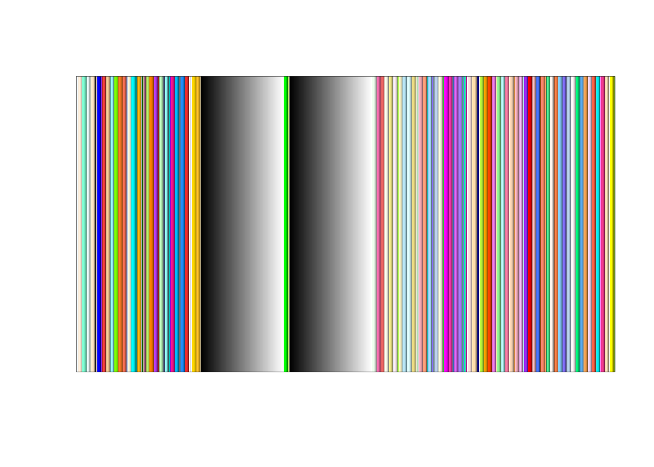
That is a lot of colors. Even at this scale, you can hopefully see that they are grouped. That is because many of the names are of the form “color#” such as “red1”,“red2”,“red3” etc. We will see this in more detail in a moment.
Let’s try a slightly cleaner panel. As an example, this is what I get when I look at the colors I use most often in these tutorials (so far):
# Check out some common colors
showpanel( c("red3", "darkblue","green3","purple"))
That is a bit more managable. Try it yourself using at least 5 colors that you are interested in. Note that I had to use the c() function (concatenate) to give more than one color, and that each color is enclosed in quotes.
9.5 Using grep to search colors
So far so good. But, what if we really want to pick a nicer blue? Do any of you really want to scroll through the list of 657 colors and type out every single blue? Yeah, neither do I. Luckily, we can use grep() for that.
grep() is a function that has its roots way back in 1973 with early version of Unix[*] The name derives from the three separate commands that previously were need to accomplish the task in the program ed: ‘g/re/p’ for ‘globally search a regular expression and print’. . It is an incredible tool on all *nix computers, though Windows as a few related tools. In all of its incarnations grep searches for a pattern and returns information about things that match it. In R, this works by searching for partial matches and returning the index of hits. In action, it looks like this:
# Example grep
grep(pattern = "w",
     x = c("a","b","w","wa","WWW") )
## [1] 3 4Note that it is case sensitive (it didn’t match “W”), and that it tells us where the matches are. This can be really handy if we want to identify which values, of example if we are using this to index a variable (such as if we wanted to separate out Types of hotdogs that have the letter “e” from those that don’t).
However, often, we want to acutally get the value itself back (and this is how grep works in other systems by default). For that, we can set the value = argument to TRUE:
# Return value
grep(pattern = "w",
     x = c("a","b","w","wa","WWW"),
     value = TRUE)
## [1] "w" "wa"Now, let’s return again to picking out a good blue. Tell grep() to match “blue” in the colors() to see all of the colors with blue in their names.
# Use grep for color picking
grep("blue", colors(), value = TRUE)
## [1] "aliceblue" "blue" "blue1"
## [4] "blue2" "blue3" "blue4"
## [7] "blueviolet" "cadetblue" "cadetblue1"
## [10] "cadetblue2" "cadetblue3" "cadetblue4"
## [13] "cornflowerblue" "darkblue" "darkslateblue"
## [16] "deepskyblue" "deepskyblue1" "deepskyblue2"
## [19] "deepskyblue3" "deepskyblue4" "dodgerblue"
## [22] "dodgerblue1" "dodgerblue2" "dodgerblue3"
## [25] "dodgerblue4" "lightblue" "lightblue1"
## [28] "lightblue2" "lightblue3" "lightblue4"
## [31] "lightskyblue" "lightskyblue1" "lightskyblue2"
## [34] "lightskyblue3" "lightskyblue4" "lightslateblue"
## [37] "lightsteelblue" "lightsteelblue1" "lightsteelblue2"
## [40] "lightsteelblue3" "lightsteelblue4" "mediumblue"
## [43] "mediumslateblue" "midnightblue" "navyblue"
## [46] "powderblue" "royalblue" "royalblue1"
## [49] "royalblue2" "royalblue3" "royalblue4"
## [52] "skyblue" "skyblue1" "skyblue2"
## [55] "skyblue3" "skyblue4" "slateblue"
## [58] "slateblue1" "slateblue2" "slateblue3"
## [61] "slateblue4" "steelblue" "steelblue1"
## [64] "steelblue2" "steelblue3" "steelblue4"That is a lot of blues. Let’s take a look at them. Note that we can just use the output of grep() directly in showpanel()
# Plot blues
showpanel( grep("blue", colors(), value = TRUE))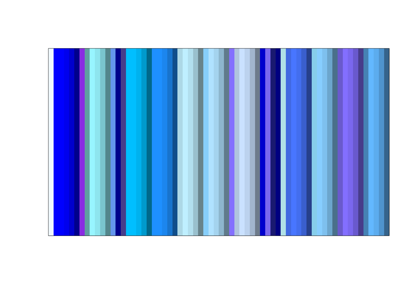
Note that the colors go in the same order as the list that was printed. Maybe we decided we like the “dodgerblue” set – we can narrow down to just those by being more specific in the pattern we search for.
# Narrow our search
grep("dodgerblue", colors(), value = TRUE)
## [1] "dodgerblue" "dodgerblue1" "dodgerblue2" "dodgerblue3" "dodgerblue4"showpanel( grep("dodgerblue", colors(), value = TRUE))
9.5.1 A note on regular expressions
grep() works by searching something called “regular expressions.” These are special ways of searching that allow you to match general patterns in addition to the normal strings we have been using. There are a lot of these special options, but most are beyond what we need to do introductory statistics. If you want to learn more, google for regular expressions, or check out this quick guide.
For our purposes, we only need to consider two of these special characters. The carat (^), which means “the start” and the dollar sign ($), which means “the end.”
So, if we just want the “basic” blue colors, we can tell R that we only want the “blue”s that occur at the start of the line like this:
# Get only the start of lines
grep("^blue", colors(), value = TRUE)
## [1] "blue" "blue1" "blue2" "blue3" "blue4"
## [6] "blueviolet"showpanel( grep("^blue", colors(), value = TRUE))
Which can be interpretted as: “give me things that match: (start of line)blue”. We can similarly pull out all of the non-numbered blues by only matching things that end in “blue”:
grep("blue$", colors(), value = TRUE)## [1] "aliceblue" "blue" "cadetblue"
## [4] "cornflowerblue" "darkblue" "darkslateblue"
## [7] "deepskyblue" "dodgerblue" "lightblue"
## [10] "lightskyblue" "lightslateblue" "lightsteelblue"
## [13] "mediumblue" "mediumslateblue" "midnightblue"
## [16] "navyblue" "powderblue" "royalblue"
## [19] "skyblue" "slateblue" "steelblue"showpanel( grep("blue$", colors(), value = TRUE))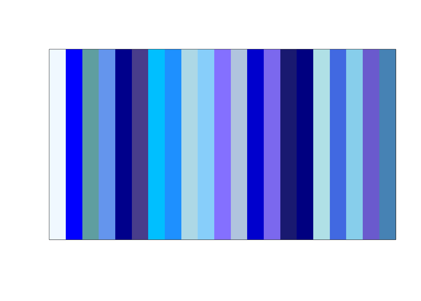
Which can be interpretted as: “give me things that match: blue(start of line)”.
9.5.2 Try it out
Now, give it a shot. Use these tools to look look at a color that interests you in R.
9.6 Picking “good” colors
In addition to these built in colors, there are lots of ways to specify colors in R. However, one of the trickiest parts is specifying good colors. This is particularly a problem for identifying colors that go well together.
Luckily, other people have put a lot of effort into developing just such color sets. There is a great web resource called ColorBrewer that has really nice sets of colors that have been vetted to work well. Do check out the website, as the interactive tool is really helpful. Luckily for us, this is also available directly within R as the package “RColorBrewer”. Let’s install and load the package:
# Install the package
install.packages("RColorBrewer")

# Load the package
library(RColorBrewer)
Don’t forget to comment out the install line to avoid accidentally re-installing.
This package comes with some great tools, including a way to view all of its built in color sets: the function display.brewer.all()
# Look at all the colors
display.brewer.all()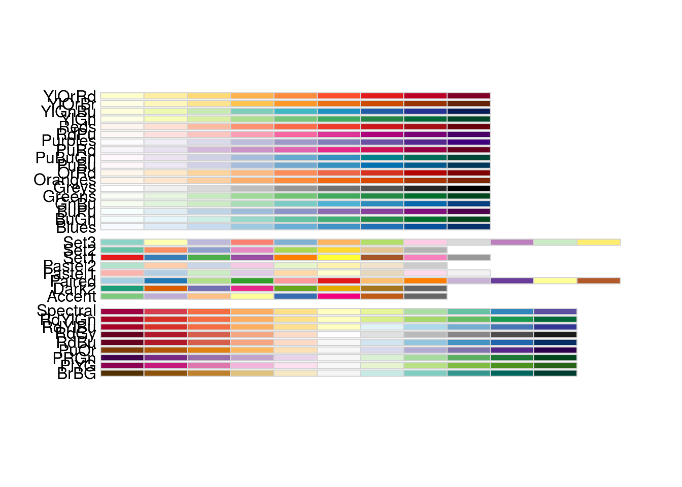
Note that this plot can be a bit messy, especially if your plot window is small. To accomodate this, we can break the plot up into three different plots, separated by the different types of color sets:
- “div” is for “diverging” colors
- “qual” is for “qualitative” colors (i.e., very different for each, which is usually what we want)
- “seq” is for “sequential” which can be useful for ordered data
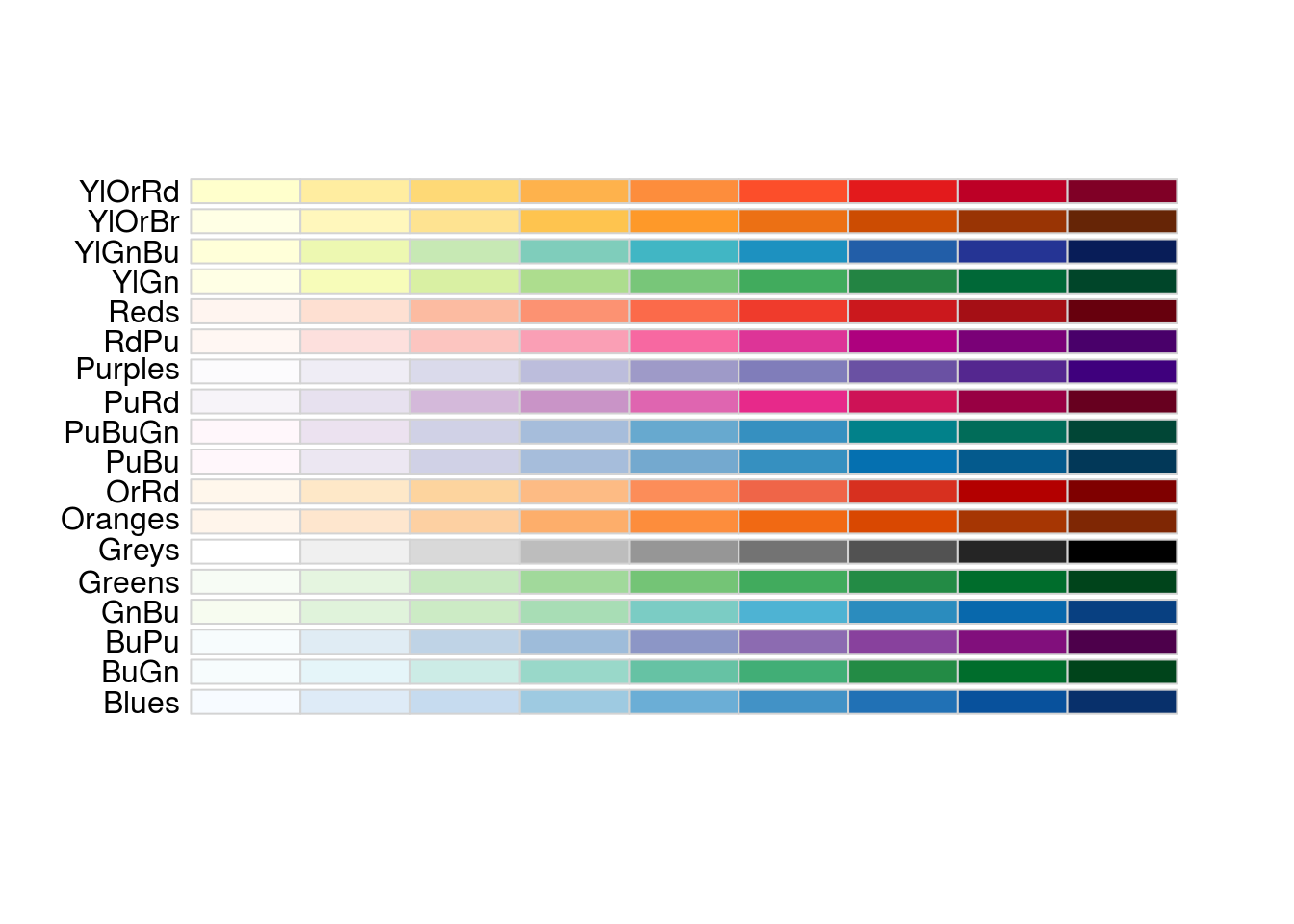
# Limit to certain types
display.brewer.all(type = "div")
display.brewer.all(type = "seq")
display.brewer.all(type = "qual")

The color sets are also specifically chosen to return a specific subset if you are using fewer than the full number of colors. We can see this by setting the n = parameter:
display.brewer.all(type = "qual", n = 5)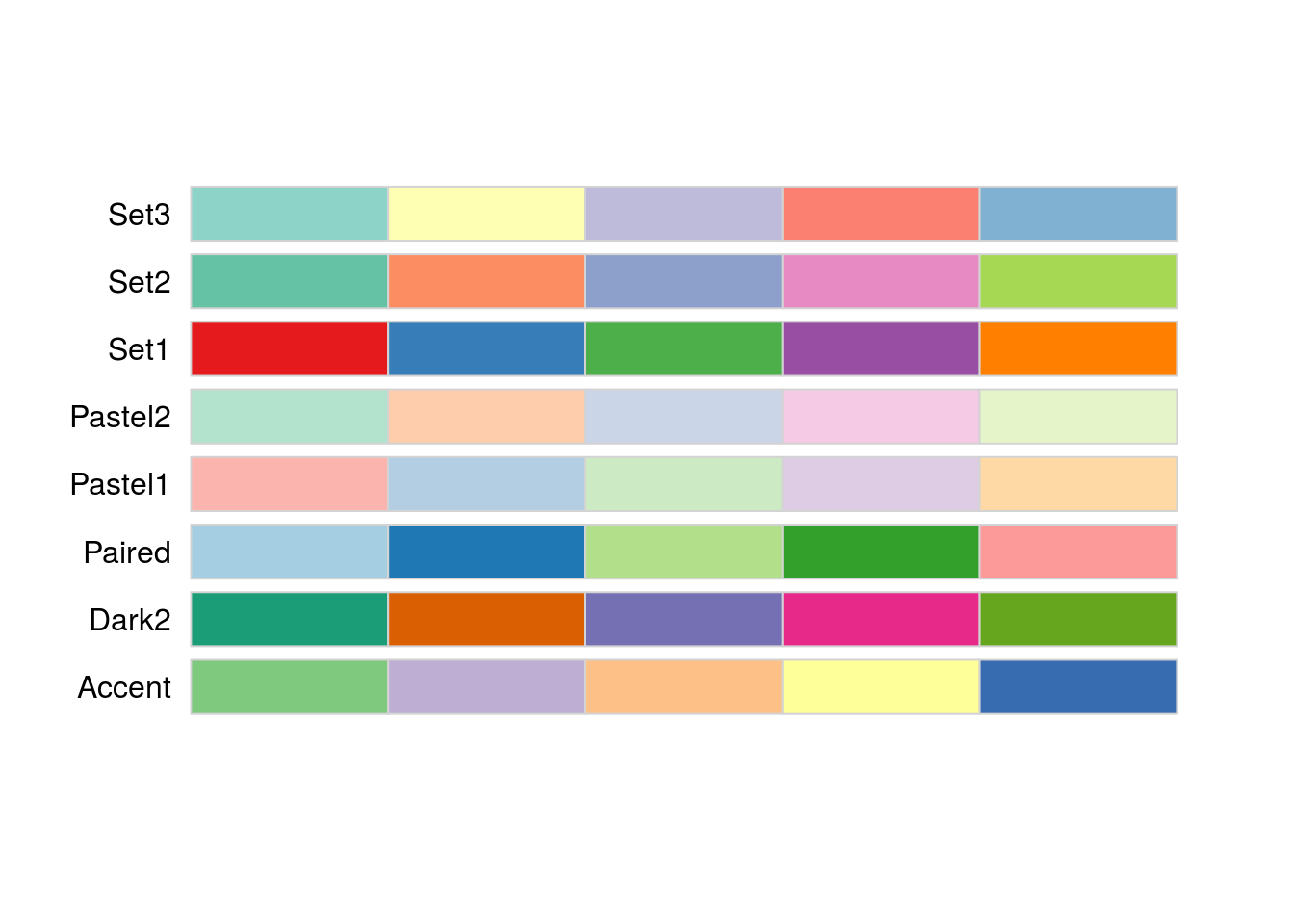
But what we really need is to get the colors out of the function so that we can use them. For that, we turn to the function brewer.pal which takes an arguement for the number of colors to return and the set to select from. Here, I am going with 3 colors from “set1”.
# Save colors
myColors <- brewer.pal(n = 3, name = "Set1")
myColors
## [1] "#E41A1C" "#377EB8" "#4DAF4A"Note here that the colors are stored as hexadecimal values[*] If you are interested, it is called hexadecimal because it is a base 16 system. each ‘digit’ ranges from 0 to F, where the letters keep counting past 9. For example, ‘A’ means 10 and ‘F’ means 15. . This is the way that most colors on the internet are saved as well, and make it possible to specify virtually any color. For example, this site list team colors for every major sports team in the US. We could use those hex colors directly.
But, for now, let’s focus on these. We can use showpanel() to confirm that they work:
# Confirm my colors
showpanel(myColors)
9.7 Using colors
To round things out, let’s see how we would actually apply these colors in practice.
9.7.1 Scatterplot
To start, we can use the code from the linear regresion chapter to see the colors in action. Here, instead of having to type out the colors, we’ve just used the myColors variable to set the colors. This is especially nice if we want to be able to change the colors easily and/or use them in multiple plots.
# Make column for colors
hotdogs$colorType <- factor(hotdogs$Type,
                            labels = myColors)

# Plot the data, setting col = to be the colors we created
# note that we have to use as.character, because otherwise
# the order of the types is returned
plot(Calories ~ Sodium, data = hotdogs,
     col = as.character(colorType),
     pch = 19)

# Add a legend, here by using levels() to make sure our orders match
legend("topleft",
       inset  = 0.01,
       legend = levels(hotdogs$Type),
       col    = levels(hotdogs$colorType),
       pch    = 19)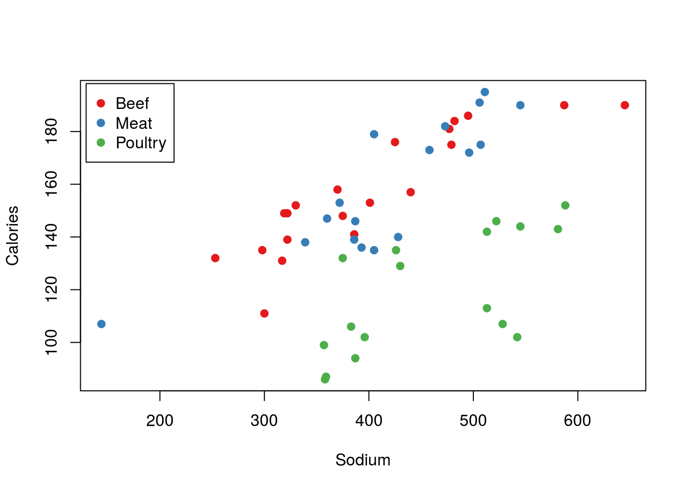
9.7.2 Simple barplot
Speaking of using colors again, let’s use these colors to make a barplot. Whenever you are presenting data, you want colors to mean the same thing throughout. So, we want to use myColors again to set the colors.
First, let’s make a plain barplot, like we have before:
# Make a table of hotdog types
typeCounts <- table(hotdogs$Type)

# Make a barchart
barplot(typeCounts,
        xlab = "Hotdog type",
        ylab = "Number of Hotdogs",
        main = "What's in your hotdog?")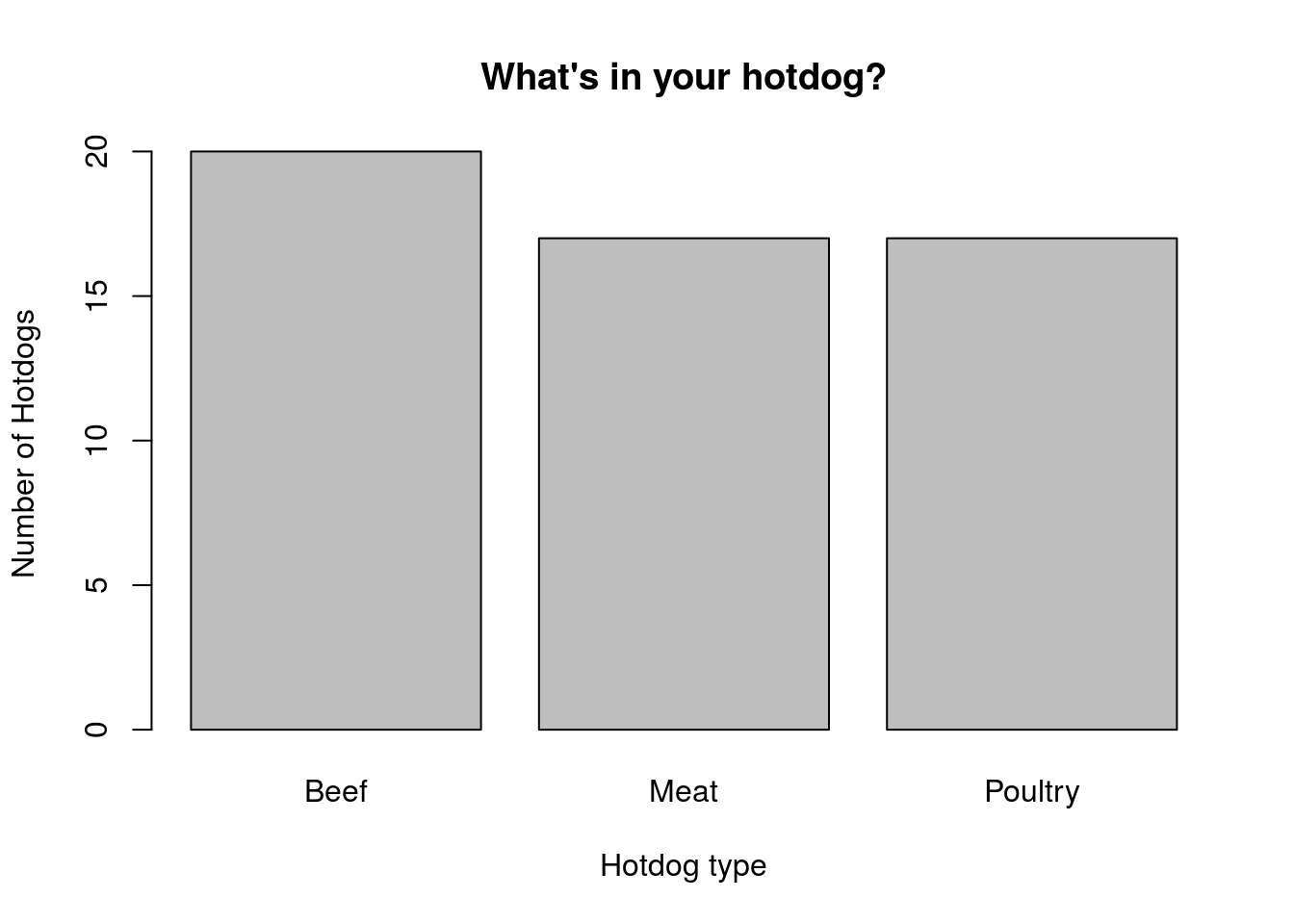
But, we’d like to use some color here. barplot() also has a col = argument, which will be used for the bars in order. We can either make the bars all the same color, like this:
# One color bar
barplot(typeCounts,
        xlab = "Hotdog type",
        ylab = "Number of Hotdogs",
        main = "What's in your hotdog?",
        col = "darkblue")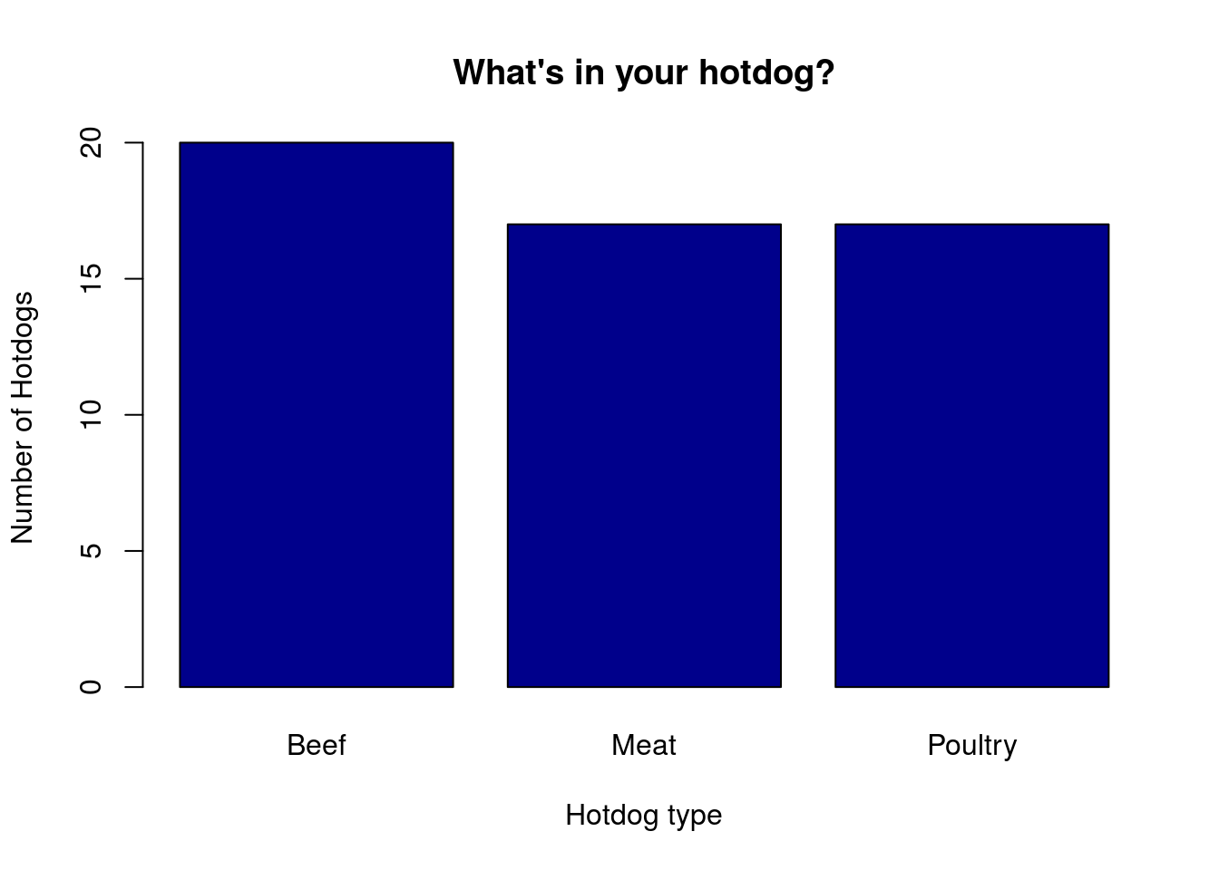
Or, we can make each bar its own color:
# Color by type
barplot(typeCounts,
        xlab = "Hotdog type",
        ylab = "Number of Hotdogs",
        main = "What's in your hotdog?",
        col = myColors)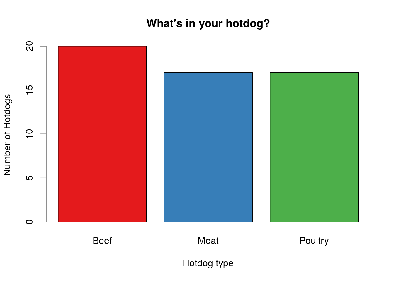
Because the bar plot is always made in the order of the levels, these colors match the ones we used on the scatter plot
9.7.2.1 Try it out
Go back and change the colors selected in myColors to something you like, and make the plots again.
9.7.3 Two way barplots
When we have two different categorical variables, sometimes we just want to use color to highlight the differences between them. For this, we turn again to the titanicData. Make a base bar plot like we have before:
# Save a two-way table of survival
survivalClass <-  table(titanicData$survival,
                        titanicData$class)
barplot(survivalClass,
        beside = TRUE,
        ylab = "Number of passengers",
        xlab = "Class",
        legend.text = TRUE)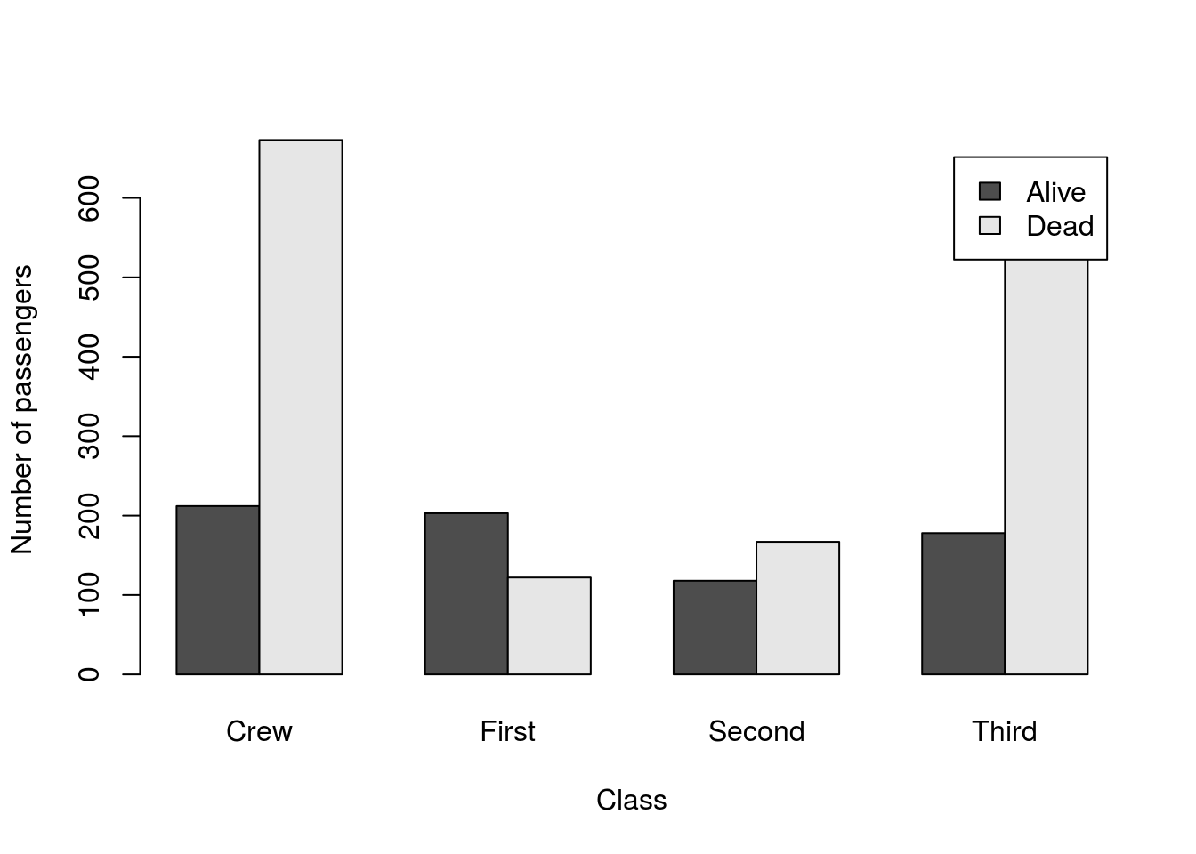
This clearly separates the survivors by color, but perhaps not the color we want. Here, we don’t need to create a new factor, we just need to tell R which colors we are using.
Here, I am going to pick out two different colors, but you should feel free to pick out any you would like. Note, however, that RColorBrewer only wants to return 3 or more colors. To get just two, I always set my values to 3, then select the first two with square brackets, though you could also select the second 2, or use a larger set and select any two you wanted (or just pick two colors a different way).
# Pick new colors
twoBarColors <- brewer.pal(3, "Dark2")[1:2]

# Change the colors
barplot(survivalClass,
        beside = TRUE,
        ylab = "Number of passengers",
        xlab = "Class",
        legend.text = TRUE,
        col = twoBarColors )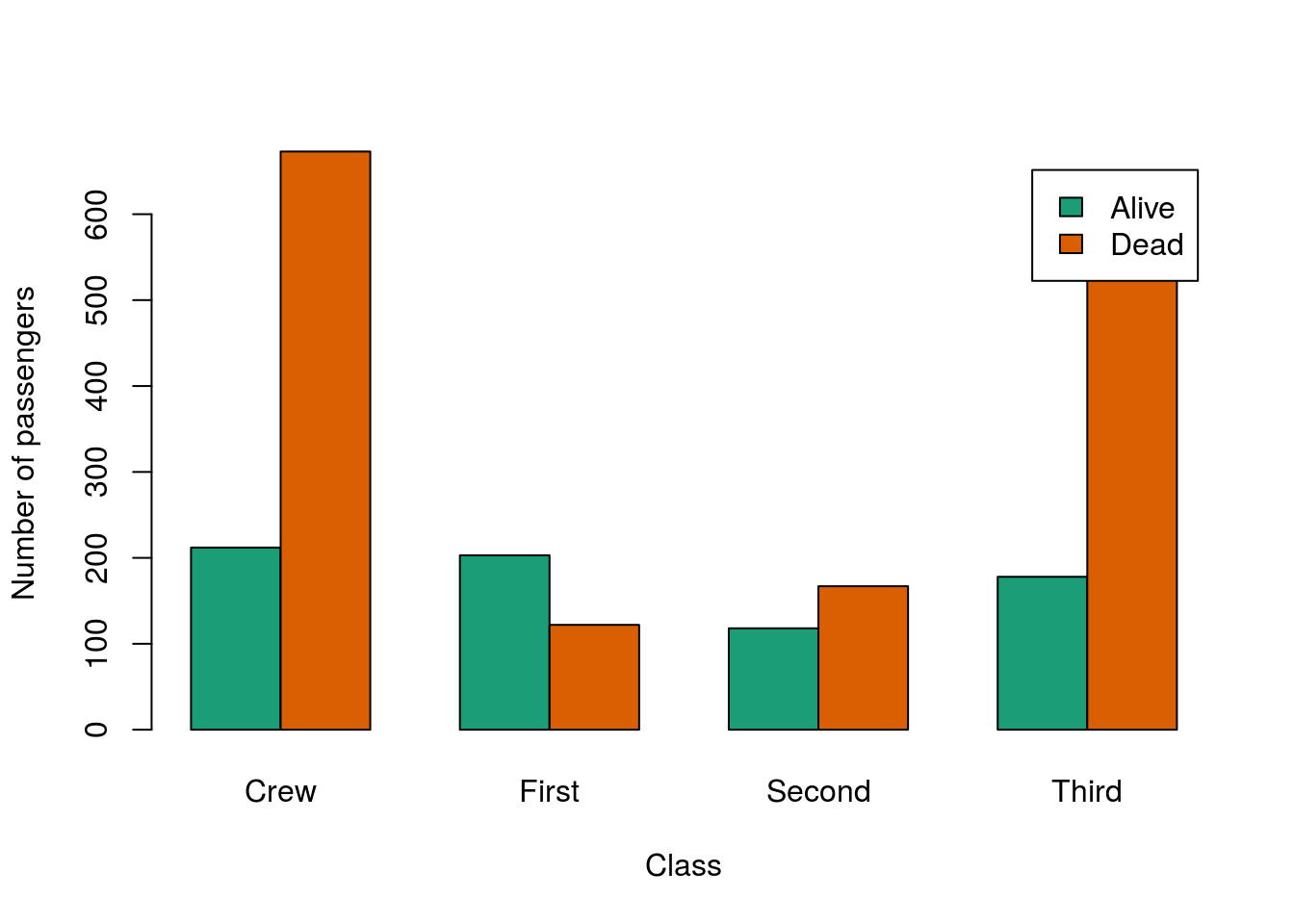
9.7.4 More complex two bars
Sometimes, we may want to get even fancier and color every single bar a different color. This isn’t neccesarily a good idea, as to many colors can be distracting. However, if you are using distinct colors throughout a report, it may make sense to continue that in the barplot.
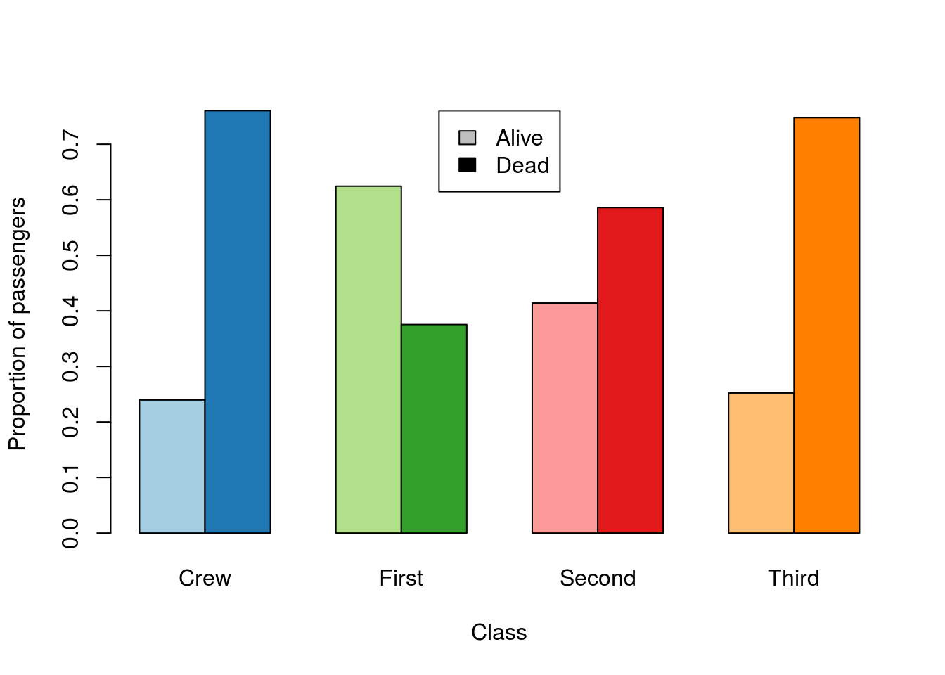
For this, let’s plot the relative survival in each class.
# Change the colors
barplot(prop.table(survivalClass,2),
        beside = TRUE,
        ylab = "Proportion of passengers",
        xlab = "Class",
        legend.text = TRUE)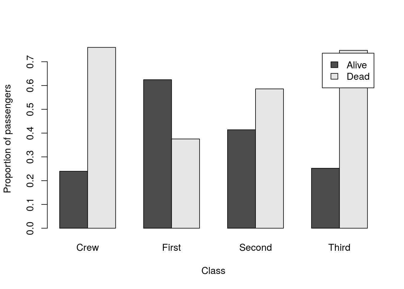
Here, we probably want paired colors. So, I am going to select a set of paired colors.
# Pick some paired colors
pairedColors <- brewer.pal(8, "Paired")

# Show what I picked
showpanel(pairedColors)
Now, if I use those in barplot:
# Change the colors
barplot(prop.table(survivalClass,2),
        beside = TRUE,
        ylab = "Proportion of passengers",
        xlab = "Class",
        col = pairedColors)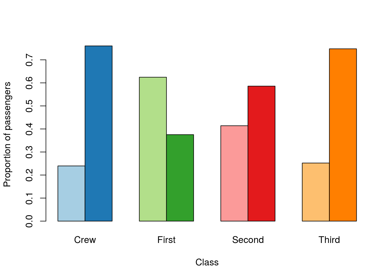
Now, each light bar is the passengers that lived, and the dark bar is those that died. Choosing paired colors is extra tricky, but see if you can manage to select a different set (hint: using square brackets may help).
Finally, we probably want a legend. For this, I am going to choose to use gray and black, and then explain (elsewhere) that all of light are living and dark are dead.
legend("top",
       legend = levels(titanicData$survival),
       fill = c("gray","black"))