11.1 Load today’s data

Start by loading today’s data. If you need to download the data, you can do so from these links, Save each to your data directory, and you should be set.

• NFLcombineData.csv
  • Data on the Height, Weight, and position type of all 4299 players that participated in the NFL combine during the collection period
• mlbCensus2014.csv
  • Basic data on every Major League Baseball player on a 25-man roster as of 2014/May/15

# Set working directory
# Note: copy the path from your old script to match your directories
setwd("~/path/to/class/scripts")

# Load data
nflCombine <- read.csv("../data/NFLcombineData.csv")
mlb        <- read.csv("../data/mlbCensus2014.csv")

11.2 What is a confidence interval?

You have all likely seen confidence intervals many times before, whether you recognized them or not. Every report on a public opinion poll lists the results as an estimate ± some error. Here, the “±” means that the actual value is likely within that amount of error of the estimate. The amount of error is generally referred to as the “margin of error” The formal form of this is:

point estimate ± margin of error

So, if a poll from the Washington Post (2014) finds that 59% of Americans (± 3.5 percentage points) support marriage equality, that means that the researchers believe that the true value is somewhere between 55.5% and 62.5%.

The same approach can be used for estimates of means. For example, a scientific study may say that the mean time that college students spend studying per week is 15 hours ± 0.5, meaning they believe the true value is between 14.5 and 15.5 hours.

But: how can they know that? In the last chapter we showed that, given a population, we can get a pretty good idea about where the samples are going to fall. When we run a poll (or collect any sample), however, we can not know what the true population looks like.

As we will see here today though, when we do know the population and the sampling distribution is roughly symmetric and unimodal, we can use the 95% rule (the fact 95% of data values fall withing 2 standard errors of the mean) as a guide.

By reversing our thinking, that means that any point estimate of a sample is likely to be inside of that range. While we will not always know which direction (or by how much) a particular sample is off by, we can use this guiding principle to state how confident we are are in our prediction.

The ranges listed above are thus called “confidence intervals” because researchers are 95% confident that the true population value falls somewhere within that range.

11.3 Calculating CI of a mean

Let’s take a lot of samples of the weights of NFL combine participants to examime our confidence in any one sample. Start by collecting samples much like we did in the last chapter.

# See where we should be
mean(nflCombine$Weight)

## [1] 245.8232

# Generate several samples
nflSamples <- numeric()
for(i in 1:1000){
  # Copy the sampling from above
  tempWeight <- sample(nflCombine$Weight,
                       size = 40)
  
  # save the mean in the "ith" position, hence index
  nflSamples[i] <- mean(tempWeight)
}

# plot results
hist(nflSamples)
abline(v = mean(nflCombine$Weight),
       col = "red3", lwd = 3)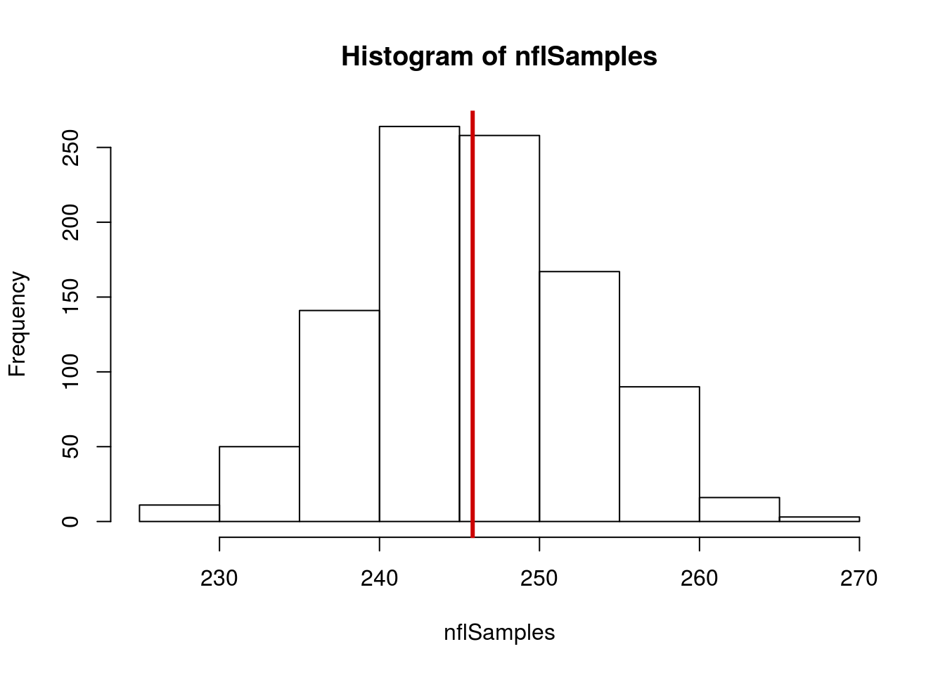

Recall that the standard error is a good metric of the spread of our distribution. So, let’s calculate it along with the mean.

mean(nflSamples)

## [1] 245.8099

sd(nflSamples)

## [1] 7.05302

Of note: the numbers here are likely to be different than yours. That is because of the random sampling – we don’t expect to get exactly the same random samples. In fact, the exact values you get when you compile to html will be slightly different than when you run it directly[*] The function set.seed() will be introduced soon, but is a bit much to cover just here. It also requires running it consistently, which is difficult to instill. .

Our standard error is 7.03 around a mean of 245.96. Recalling the 95% rule (that 95% of data of data are within 2 SE of the mean) this indicats that, assuming a normal distribution, 95% of our estimates fall between about 232 and 260 pounds

We can, however, turn this on its head. Because we know that about 95% of our samples are within that range, that also means that, from our samples, the mean is within 2 SE (7.03) of our sample mean for about 95% of our values.

Here each point represents one of the samples taken (an illustrative subset). The bars around each represent 2 SE’s away from that point estimate in either direction (like what we would calculate if we only had a sample, not the population). Finally, the lines represent the population mean (which we know because we have the whole population) and the “fences” representing 2 SE in either direction.

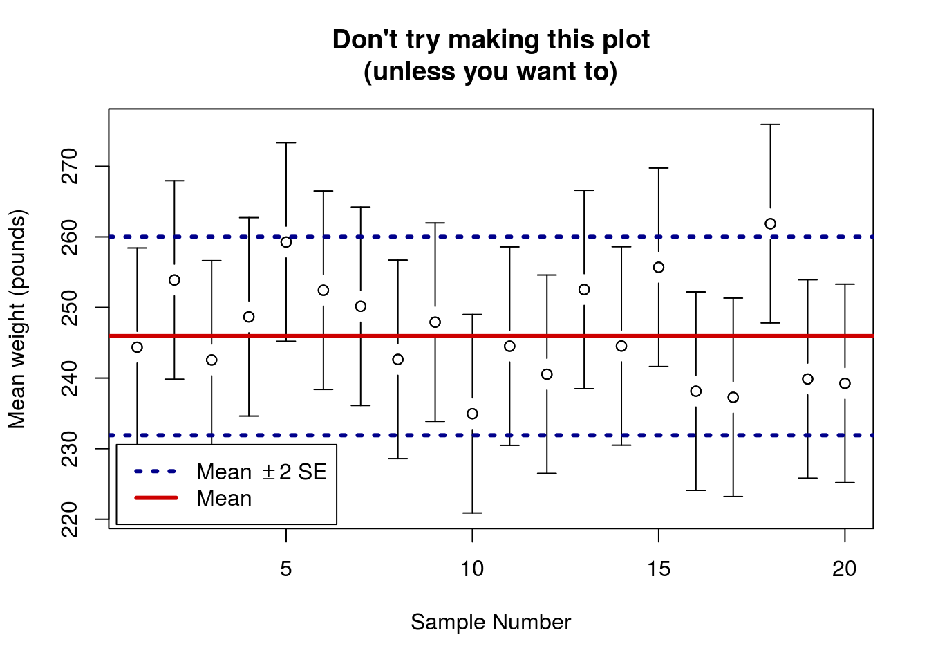
There are two things to note here: First, even though all of the samples came from the population, one of the does fall outside of our expected range. This is exactly what we expect! About 95% (or 1 in 20) of the estimates should fall outside of 2 SE. Second, the length of the bars is exactly the same as the distance between the mean and 2 SE cutoffs. This means that, if the sample falls within 2 SE of the mean, then the mean will be within 2 SE of the sample.

Ok – that sounds funny, but it is important. Usually, we won’t have the population parameters handy, so we won’t know whether or not we are close to the “true” value. However, we can figure out how far away we expect the mean to be.

Said another way, if you had collected the first sample on the graph, (but didn’t know what the true value was) you would say that you were 95% confident that the true value was between 230.32 and 258.43 pounds (the ends of the bars). If, instead you had collected the 18th sample (3rd from the right) you would say that you were 95% confident that the true value was between 247.82 and 275.93 pounds. In the latter case, your confidence interval would not contain the true mean (246).

This does not mean that you did anything wrong. Errors like this are just one of the costs of making estimates like this. In a later tutorial, we will explore how to balance these errors while still being able to say something about the population.

One thing that we can do is to check how often the true mean really is within 2 standard errors of your samples. First, simply ask how many are within our 2 SE above and 2 SE below the mean fences. Note that this kind of a logical works just like others we have encountered before. The only difference is that when we use the & the value must meet both criteria that we set.

# Ask if each sample is less than 2 sd above AND
#   more than 2 sd below the mean
# Note that I broke this over several lines for readability
# IF you do the same, make sure to break at place where it
# is clear to R that you want to keep reading the next line
isClose <- nflSamples < mean(nflCombine$Weight) +
                          2*sd(nflSamples) &
           nflSamples > mean(nflCombine$Weight) -
                          2*sd(nflSamples)

# See what the output looks like
head(isClose)

## [1] TRUE TRUE TRUE TRUE TRUE TRUE

Now, we can treat those TRUE and FALSE values just like 1’s and 0’s. First, count how many TRUE are in the variable isClose (this is the number within 2 SE).

# See how many fall within
sum(isClose)

## [1] 952

Next, we want to know the proportion that represents. So, we divide by how many values are in isClose, which is what is returned by length()

# See the proportion that fall inside
sum(isClose)/length(isClose)

## [1] 0.952

That looks an awful lot like a mean. Turns out we can just use mean(), as it internally does the same calculation.

# Quicker
mean(isClose)

## [1] 0.952

Here, we see that about 95% of our values (95.2% to be specific) are within two standard errors.

11.4 Calculating CI of a proportion

This doesn’t just work for means. Instead, we can use a sample to calculate just about any metric, and determine the range that we believe, with 95% confidence, contains the real value.

What proportion of combine participants are skill players? Calculate the true proportion. Here, we aske “Does the column equal skill”, then calculate the proportion of the values that are TRUE.

# Calculate what proportion are skill players
mean(nflCombine$positionType == "skill")

## [1] 0.662247

Now, let’s draw a sample of 100 players and see what we get.

# get a sample
tempPos <- sample(nflCombine$positionType, 100) 

# calculate the proportion
mean(tempPos == "skill")

## [1] 0.7

This gives us a proportion of 0.7, very close to the true proportion.

Now, lets try drawing more samples

# Generate several samples
nflSampleProps <- numeric()
for(i in 1:1000){
  # Copy the sampling from above
  tempPos <- sample(nflCombine$positionType, 100) 

  # save the proportion in the "ith" position, hence index
  nflSampleProps[i] <- mean(tempPos == "skill")
}

mean(nflSampleProps)

## [1] 0.66192

sd(nflSampleProps)

## [1] 0.048665

This shows us that our mean is very close to the actual, and gives us a standard error of 0.049. We can use that to show that we expect about 95% of our samples are within 0.097 (2 SE) of the true proportion

# Store the true proportion
trueProp <- mean(nflCombine$positionType == "skill")

# Ask if each sample is less than 2 sd above AND
#   more than 2 sd below
isClose <- nflSampleProps < trueProp +
                              2*sd(nflSampleProps) &
           nflSampleProps > trueProp - 
                              2*sd(nflSampleProps)

# See what the output looks like
head(isClose)

## [1] TRUE TRUE TRUE TRUE TRUE TRUE

# See how many fall within
sum(isClose)

## [1] 960

# See the proportion that fall inside
mean(isClose)

## [1] 0.96

Again, about 95% of our samples are within 2 standard errors of the true proportion.

11.5 Try it out

Create a sampling distribution of the Height’s of MLB players. What proportion of these samples do you expect to fall within 2 SE of the population mean?

11.6 What a confidence interval is not

A confidence interval is a fantastic tool for helping us fairly estimate population parameters from a sample. However, for a number of reasons, there are a few misconceptions about them. These statements show some of the most common misconceptions, each of which is incredibly common in students first learning about them. You must work hard to overcome these misconceptions.

A confidence interval does not contain 95% of the data values. We can see this clearly if we plot our sampling distribution along with the distribution from the population:

par(mfrow = c(2,1))
hist(nflSamples,
     main = "Sample Means",
     xlab = "Sample mean weight (pounds)",
     xlim = c(140,400))
hist(nflCombine$Weight,
     main = "Individual Values",
     xlab = "Weight (pounds)",
     xlim = c(140,400))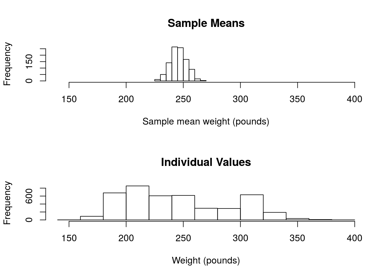

While the 95% confidence interval we calculated is between 232 and 260 pounds, our actual values extend well beyond that.

In addition, the confidence interval does not predict where the value of another sample will fall. Even if your your confidence interval does contain the true value, the next sample may, by chance, fall in the other direction from the true value. Again, we can see this by looking at the samples:

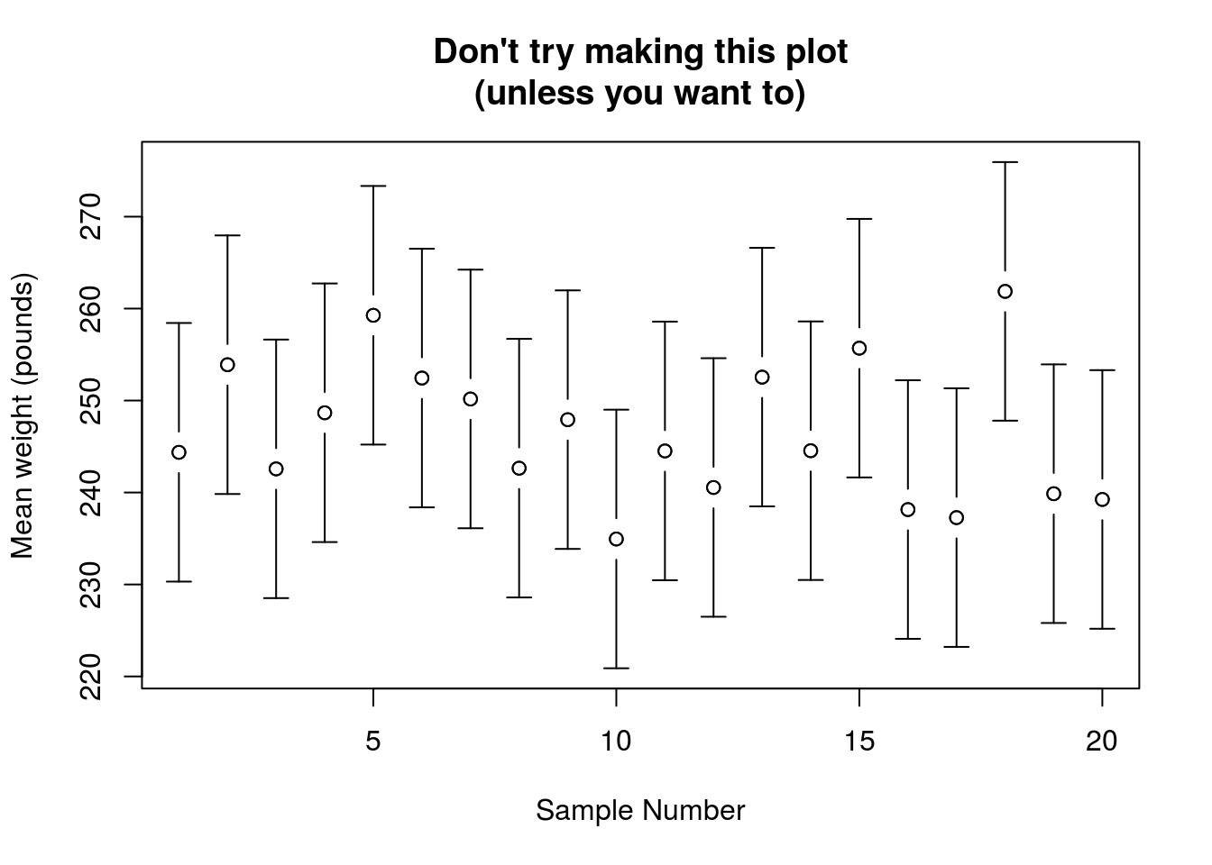
Note that many of the dots (the sample values) fall outside of the confidence interval of the samples near them.

11.7 A note on where we are going

How often, in the real world, can you collect 1000 sample to determine the standard error? Almost never!

In reality, we need to estimate the standard error, and that is where we are going in the next tutorial.