An introduction to statistics in R
A series of tutorials by Mark Peterson for working in R
Chapter Navigation
- Basics of Data in R
- Plotting and evaluating one categorical variable
- Plotting and evaluating two categorical variables
- Analyzing shape and center of one quantitative variable
- Analyzing the spread of one quantitative variable
- Relationships between quantitative and categorical data
- Relationships between two quantitative variables
- Final Thoughts on linear regression
- A bit off topic - functions, grep, and colors
- Sampling and Loops
- Confidence Intervals
- Bootstrapping
- More on Bootstrapping
- Hypothesis testing and p-values
- Differences in proportions and statistical thresholds
- Hypothesis testing for means
- Final thoughts on hypothesis testing
- Approximating with a distribution model
- Using the normal model in practice
- Approximating for a single proportion
- Null distribution for a single proportion and limitations
- Approximating for a single mean
- CI and hypothesis tests for a single mean
- Approximating a difference in proportions
- Hypothesis test for a difference in proportions
- Difference in means
- Difference in means - Hypothesis testing and paired differences
- Shortcuts
- Testing categorical variables with Chi-sqare
- Testing proportions in groups
- Comparing the means of many groups
- Linear Regression
- Multiple Regression
- Basic Probability
- Random variables
- Conditional Probability
- Bayesian Analysis
Hypothesis testing and p-values
14.1 Load today’s data
There are no data sets for today. We will be inputting a few examples of our own instead.
14.2 Overview
This chapter introduces the concept of hypothesis testing and the language associated with it. We have spent a lot of time working on how to generate a sample from a population. Here, we begin the process of using a sample to infer things about a population.
To start, we want to focus our attention a little more closely on how to generate a hypothetical sampling distribution, given an idea about what we think the should look like.
14.3 Definitions
I can not stress enough how important it is that you read this section.
The concepts here will be vital to where we go next. We will discuss them in context as they arise, but there is no substitute for understanding them now.
14.3.1 Hypotheses
14.3.1.1 Null Hypothesis
The null hypothesis, written in the notation H0, (that is an “H” with a zero subscript; pronounce “H nought”) states that there is no effect or difference, or that the mean is some set level. The null hypothesis is always a specific value (often 0), and cannot be a range of values. It must be a specific value, because we are going to use that specific value to imagine what we expect would happen if it were true.
One way to think about the null hypothesis is to think of it as the most boring thing that could be true about the data. It is the status quo, the default, the complete lack of an effect or difference. We will see these in action many times, but make sure to think through carefully.
14.3.1.2 Alternative Hypothesis
The alternative hypothesis, written Ha, is the claim that we are seeking to support, namely, that there is an effect or differnce. Said another way, the alternative hypothesis is simply that the null is not true. The alternative hypothesis is not a point estimate, but rather encompasses a range of possible values that are different than the point estimate made by H0.
14.3.1.3 Put together
It is important to remember that we always need both a null and an alternative hypothesis. If we want to know if NFL linemen are heavier than skill position players, we need a null (that they are not different weights) as well as an alternative (that they are different). It is also crucial to remember that what we are actually testing (see significance below) is how unlikely it would be to get our data (or more extreme) if the null hypothesis is true.
14.3.2 Statistical test
A statistical test is the use of a sample to assess a statement about a population.
We can know the value of a sample statistic exactly (e.g., we know that exactly 7 of the 8 beads were red), but we often don’t (and can’t) know the value of a population parameter exactly (e.g., we can’t weigh every person in the U.S). A statistical test is a way of deciding if our estimate from a sample tells us something about the population as a whole.
Specifically, for most of this course, we are going to ask how likely the data were to occur if the null hypothesis were true. We will use this information to decide about the “significance” of our result.
14.3.3 Statistical significance
When results are so extreme that we determine it is unlikely that they would have occurred if the null hypothesis is true, we say that the result it statistically significant. In this case, we “reject” H0. If we reject H0, it gives evidence to support our Ha. However, this is not a guarantee that Ha is true.
An important point here is that we never “accept” H0. Even data that perfectly match our expectations if H0 were true could have occured under some other true population parameter. A traditional null-hypothesis significance test can only reject or not reject H0 (the null).
14.3.4 P-value
Some of you may have encountered the idea of p-values before, for others, this may be your first exposure to the term. In either case, we will spend a substantial amount of time, this chapter and throughout the semester, discussing and interpretting p-values This definition is so important to everything we are doing that I am highlighting it here:
Definition of a P-value
A p-value is the probability of generating data that are as extreme as, or more extreme than, your collected data, given that the null hypothesis was true.
Put another way, a p-value is the probability that your data (or more extreme data) would have been generated by chance if the null hypothesis is an accurate description of the world. In this way, we are essentially asking how rare our data would be if the null hypothesis is true.
We care about this because it allows us to say how unexpected our data are. If they are very unlikely (have a low p-value), we can reject the null hypothesis and say that it is unlikely to be true because it is unlikely to have produced these data. We will see more about how to decide how low is low enough to make this decision in the coming chapters.
Many books and materials focus on the idea of p-values long before they show you how to generate these values. I think it is instructive to start here. So, here, we are going to focus on how to generate p-values for some simple cases, then we will spend time on interpretation throughout the next chapters.
Pay attention to these worked examples (and your assigned problems), as they are going to be very helpful to your understanding of the underlying concepts. I will endeavor to spend class time focusing on applications.
14.4 A coin-flipping example
If we think that someone might have a heads-biased coin (a coin that comes up heads more often than tails), we might want to test that hypothesis. For this, we can set our null hypothesis as a “fair” coin (one that is equally likely to come up heads or tails), and our alternative hypothesis as a probablity of heads greater than 0.5. In math notation:
H0: p(heads) == 0.5
Ha: p(heads) > 0.5
So, if we flip the coin 10 times and get 7 heads, do we think the coin is biased?
One question we can ask is how likely that result is by chance. To do that, lets flip 10,000 fair coins ten times each and see how often we get seven (or more) heads.
…
This might take a while. Let’s try R instead.
First, save the data that we collected. (Note that, if you have data in a data.frame already, this would likely mean just saving a column or subset of one.)
# Store our data
theData <- rep( c("H","T"),
                c( 7 , 3))

# Save the number of heads
nHeadsData <- sum(theData == "H")

# View the data
table(theData)
## theData
## H T
## 7 3Next, we need to draw many, many samples from our null distribution (the distribution that matches H0). The loop we make to do that should look very familiar. It is very, very similar to a bootstrap or sampling loop. The only difference is that, instead of re-sampling from our collected samples or a known population, we instead take samples from a distribution that matches our H0.
Here, that means from a coin that comes up heads and tails equally often. As with our other sampling, when we generate our samples from H0, it is very important that we use the same size as our collected data. We want to match everything we can about our sample collection method.
First, it is always a good idea to take one simple sample. This is a good way to get a sense of what is happening, and is an opportunity to catch errors that might creep into the proccess.
# Create a fair coin for sampling
fairCoin <- c("H","T")

# Generate a "test" sample
tempData <- sample( fairCoin,
                    size = length(theData),
                    replace = TRUE)
# Look at the output
tempData
## [1] "T" "T" "H" "H" "T" "T" "T" "H" "H" "H"# Count the number of heads
sum(tempData == "H")## [1] 5So, we see that we got a series of “H” and “T”, and that we can count up that we got 5 heads. All of this looks reasonable, so we can proceed with making our loop. If you were doing this yourself (instead of copying what I have below), you would likely copy your sampling lines above, and just make sure that you store the sum(tempData == "H") into a variable (that’s how I made this one).
# Initialize our variable
# Note that all we need to save is the number of heads
nHeadsSamples <- numeric()

for(i in 1: 10000){
  # Generate a sample
  tempData <- sample( fairCoin,
                      size = length(theData),
                      replace = TRUE)

  # Count the number of heads
  nHeadsSamples[i] <- sum(tempData == "H")

}

# Visualize our results
hist(nHeadsSamples,
     xlab = "Number of heads in sample",
     main = "Null distribution of 10 coin flips")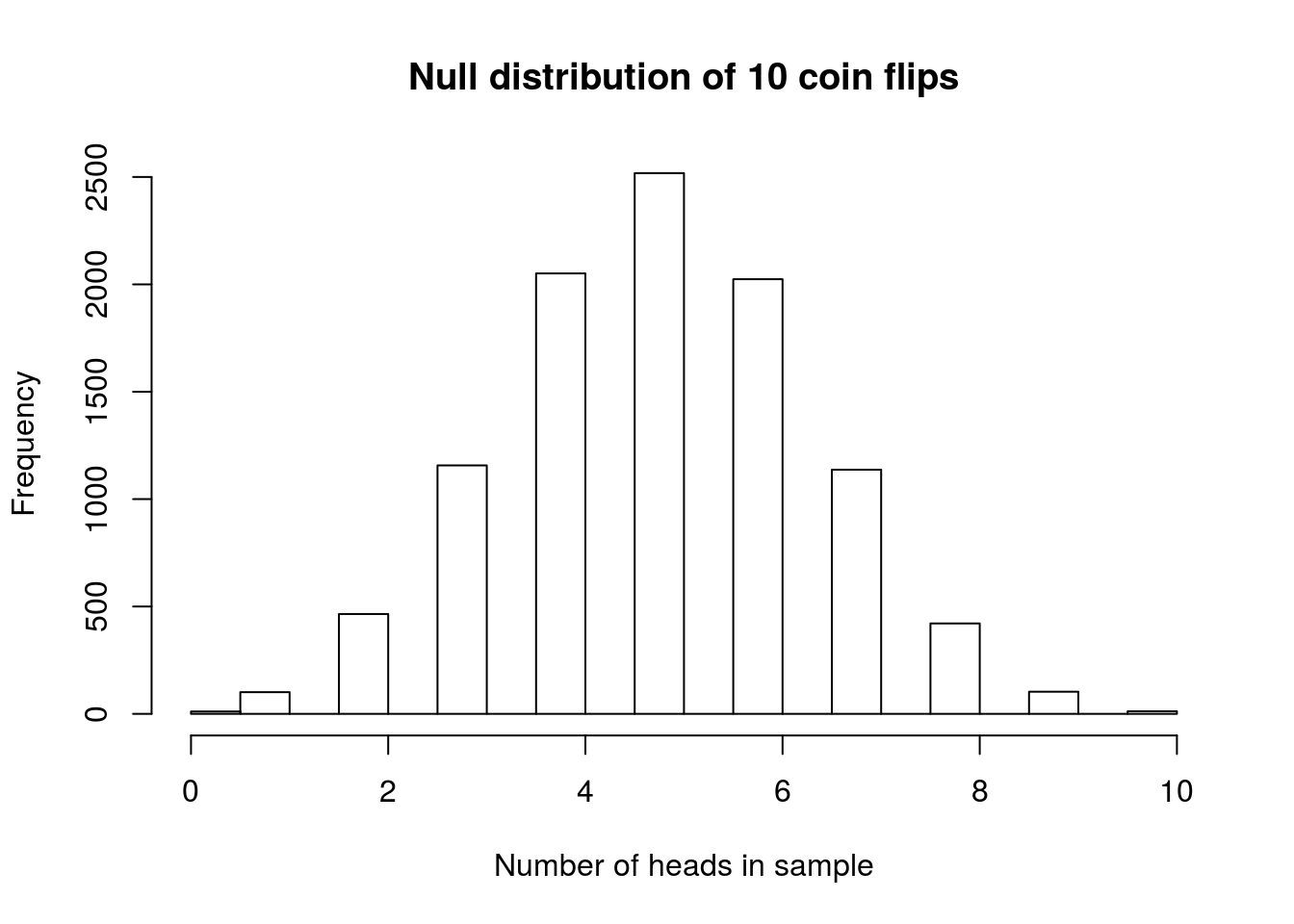
This histogram shows us a nice, unimodal, symmetric distribution. As expected, it is centered at 5 heads and 5 tails. Because the values can only range from 0 to 10, we can look at the data directly with a table. Note, however, that for many (most) data sets that is a bad idea, and that the histogram will be much more informative.
# Make a table (Note: only do this with small samples)
table(nHeadsSamples)| 0 | 1 | 2 | 3 | 4 | 5 | 6 | 7 | 8 | 9 | 10 |
|---|---|---|---|---|---|---|---|---|---|---|
| 11 | 101 | 465 | 1157 | 2051 | 2518 | 2024 | 1137 | 421 | 103 | 12 |
The first thing this shows us is that, when we flip a fair coin 10 times, it will occasionally come up all heads or all tails, just by chance.
Now that we have this, we want to calculate how likely it was to get 7 heads in 10 flips of a coin we know is fair. First, let’s add a line to the plot to show where we are looking:
abline(v = nHeadsData,
       col = "red3", lwd =3)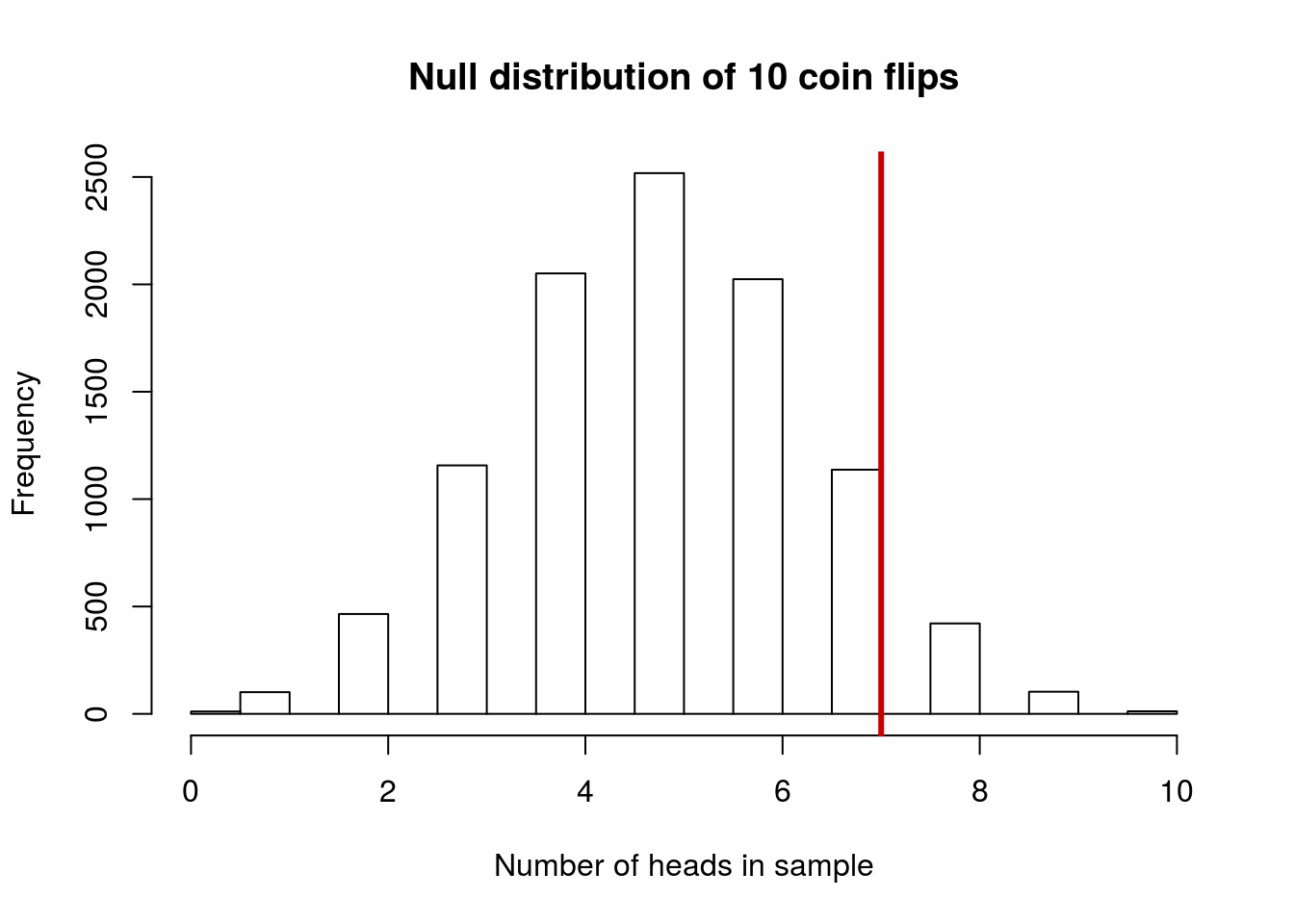
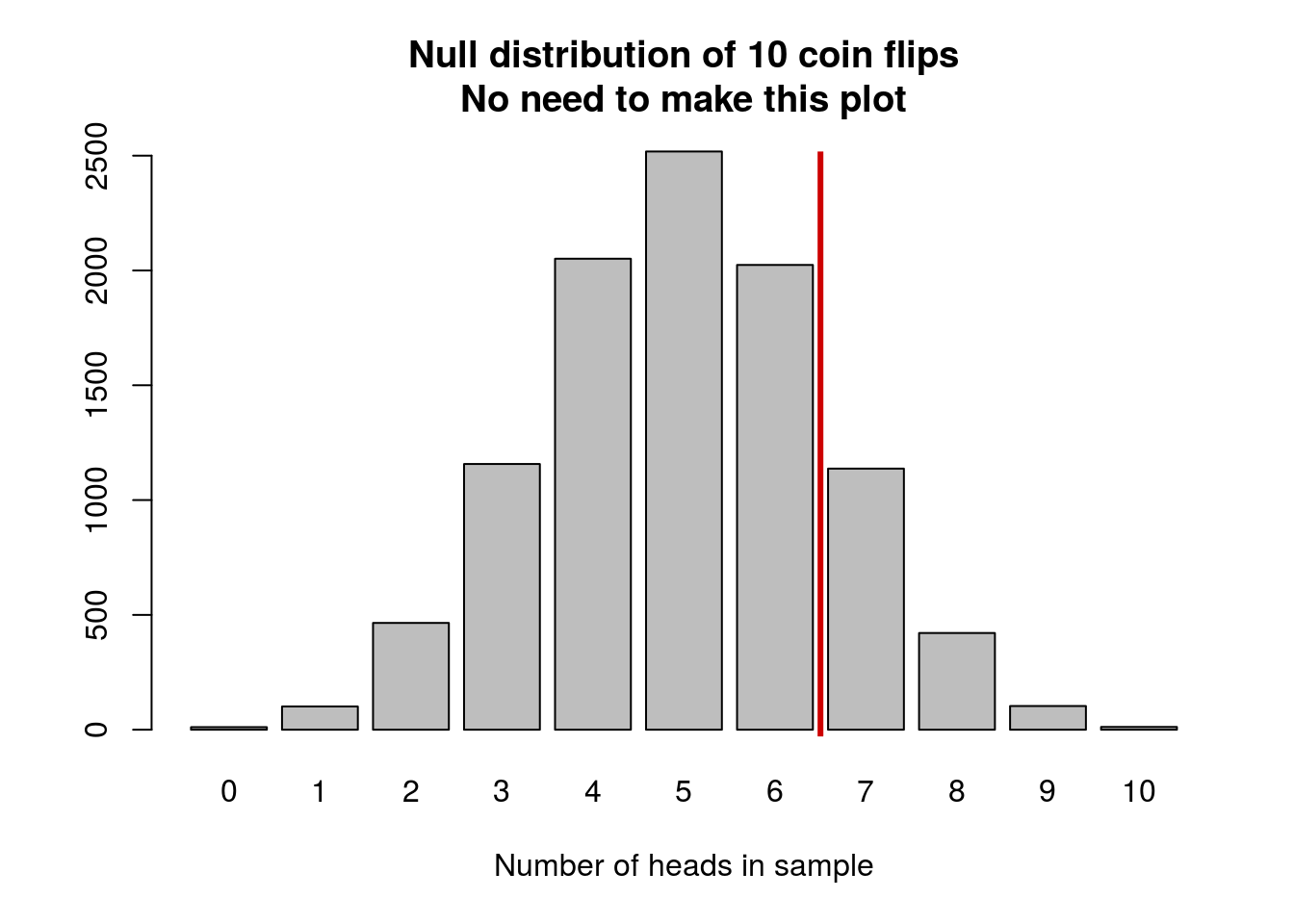
Note here that, because of the way the histogram is built, the values right at the line (i.e. 7 heads) appear in the bar just left of the line. That is ok, just make sure to keep that in mind as we consider the value we are about to calculate. An alternative plot might help in this case, though it will apply in so few situations that I do not want you to try to make this plot[*] For those of you that want to do it anyway: I did this using barplot, but barplot doesn’t put things quite where you would expect. If you save the output of barplot (e.g. spots <- barplot(table(1:3))) you can see where the bars are actually centered. This is more than you need to do for class, but if you are interested, I at least wanted to give you an explanation for why your likely first attempts would have given odd results.
What we want to figure out is how many of our samples from the null distribution gave us 7 or more heads. Recall that the p-value asks about data as extreme as, or more extreme than, the data collected. So, we get to introduce a new logical test operator, the >= for “greater than or equal to”. We count up the number that are as or more extreme, and divide by the total number. Because that is the same as calculating a mean, we can do it in one short step. However, don’t confuse this with calculating the mean of a numeric variable.
# Test likelihood of our data
propAsExtreme <- mean(nHeadsSamples >= nHeadsData)
propAsExtreme
## [1] 0.1673This suggests that we are likely to get 7 or more heads in 10 flips roughly 17% of the time we flip a fair coin. This seems fairly common (about 1 time in 6, so this probably doesn’t give us enough reason to reject the null hypothesis that the coin is fair. This does not mean that the coin is neccesarily fair; it only means that we cannot say it is not fair.
14.4.1 Try it out
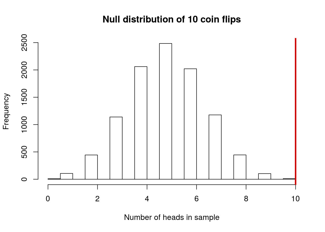
Imagine that instead of getting 7 heads in 10 flips, we had gotten 10 heads in our 10 flips. How often is that likely to have occurred by chance, if the coin is fair? What does that suggest to you? Our null and alternative hypotheses remain the same.
You should get a value of about 0.0011, though your answer will vary a bit because of the random sampling. Note that your value may be printed in scientific notation. If you get something like 11e-04, it means \(11*10^{-4}\). The number after the e is the exponent on the 10. It is just a short hand way of showing scientific notation (and is common in many programs). Don’t forget to plot your null distribution either; you should get something like this
14.5 (Sample) size matters
Just like in our other distributions (bootstrapping and sampling) e once again find that sample size matters in these tests What if, instead of flipping the coin 10 times, we flipped it 100? Imagine if we got the same proportion of heads, giving us 70 heads in 100 flips. Now, how unlikely is this.
Here, you will (hopefully) see why I used some of the variables I did above. Copy and paste all of what you just did. All we need to change is our initial data theData to have 70 heads and 30 tails, instead of 7 and 10. If instead of using length() in the loop I had typed in 10, we’d now have to change that as well.
# Store our data, for ease of access
theData <- rep( c("H","T"),
                c( 70, 30))

# Save the number of heads
nHeadsData <- sum(theData == "H")

# Create a fair coin for sampling
# Note, we use one of each face
fairCoin <- c("H","T")

#####################
# Run the full loop #
#####################

# Initialize our variable
# Note that all we need to save is the number of heads
nHeadsSamples <- numeric()

for(i in 1: 10000){
  # Copy the test sample into our loop
  #   (or build the loop around it)

  # Generate a sample
  tempData <- sample( fairCoin,
                      size = length(theData),
                      replace = TRUE)

  # Count the number of heads
  nHeadsSamples[i] <- sum(tempData == "H")

}

# Make a table (Note: only do this with small samples)
# Now it is a bad idea
# table(nHeadsSamples)


# Visualize our results
hist(nHeadsSamples)
abline(v = nHeadsData,
       col = "red3", lwd =3)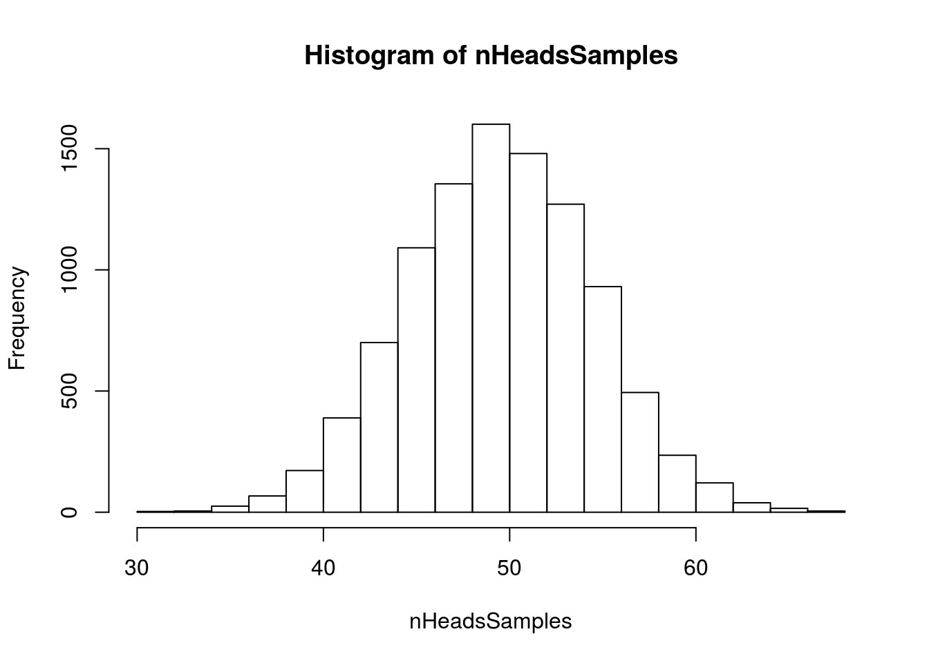
In all of this code, the only things I changed were the original data, and commenting out the table (it would be quite large). Now, again with exactly the same code, we can again test how many of our samples had as many (or more) heads
than our original sample (70).
# Test likelihood of our data
propAsExtreme <- mean(nHeadsSamples >= nHeadsData)
propAsExtreme
## [1] 0Here, I got no samples with 70 or more heads from the null distribution. In a large class, at least a few of you will get one or two. Still, with that few occurrences, we can rather comfortably say that the data (70 heads in 100 flips) were unlikely to have happened by chance if the coin were fair. So, we reject the null hypothesis, and say that we think the coin is unlikely to be fair.
14.5.1 Try it out
How likely is it to get 110 heads in 200 flips? Calculate and interpret a p-value. Don’t forget a plot.
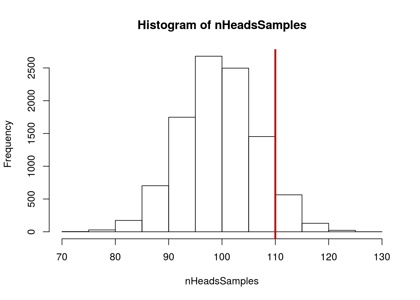
You should get a p-value of about 0.09.
14.6 Two tails?
What if, however, didn’t suspect that the coin was heads biased, but just that it might be biased? Would only checking things greater than 7 or 70 make sense?
Instead, we usually use a two-tailed test. This way, we will include the biases in both directions, rather than only one. For almost every hypothesis you test, a two-tailed test will be more appropriate. Only if you have a strong reason to expect a particular direction of difference (e.g., if Ha is greater than or less than, rather than just not equal), is a one-tailed test appropriate.
There are two ways of getting this value: doubling the one-tailed value and actually measuring both. The former is a bit simpler, but the latter is more robust to problems caused by non-symmetrical data.
For you, go back and run the example with only 10 flips, as the effects are easier to see. In most circumstances, you would want to use different variable names, so that you can keep testing both things.
And a table:
| 0 | 1 | 2 | 3 | 4 | 5 | 6 | 7 | 8 | 9 | 10 |
|---|---|---|---|---|---|---|---|---|---|---|
| 11 | 104 | 435 | 1197 | 2102 | 2417 | 2002 | 1185 | 442 | 96 | 9 |
To test the first, we can just regenerate the proportion we calculated before, and double it.
# Test likelihood of our data
propAsExtreme <- mean(nHeadsSamples >= nHeadsData)
propAsExtreme * 2
## [1] 0.3464Now, we see that such a bias is likely to occur about 1 time in 3, quite likely.
To test more formally, we can add a second value, one for below our expected values.
To do this, we first calculate how many heads we expected if the coin were fair.
# how many heads we expect
nHeadsExpected <- 0.5 * length(theData)
nHeadsExpected
## [1] 5As your intution told you, this is the middle of the null distribution. Next, we figure out how far away from that value our data were. For this, it is often best to use the absolute value, calculated using abs() in R. This way, the value is always positive, and we don’t need to worr as much about getting our directions right.
# How extreme our data are
ourDiff <- abs(nHeadsData - nHeadsExpected)
ourDiff
## [1] 2Finally, we calculate how many values are as (or more extreme) as our original sample. That is, how many were as far away, or further, from the expected value in either direction.
# Calculate the propotion that are that extreme
# in the other direction
propAsExtremeLess <- mean(nHeadsSamples <=
                            (nHeadsExpected - ourDiff) )

propAsExtremeMore <- mean(nHeadsSamples >=
                            (nHeadsExpected + ourDiff) )

# Add the two together
propAsExtremeLess + propAsExtremeMore
## [1] 0.3479This gives us a value very similar to the above, but it is a bit safer. We can look at the values separately to see why this might be the case:
| propAsExtremeLess | propAsExtremeMore |
|---|---|
| 0.1747 | 0.1732 |
While the values are very similar, there are slight differences. In more complicated analyses, these differences may be meaningful.
14.6.1 Try it out
Calculate the two-tailed p-value for the example above with 105 head in 200 flips.
14.7 A note on significance thresholds
We can all probably agree that 7 out of 10 heads is not extreme enough to reject our null, but that 70 out of 100 is. Somewhere between these two extremes lies a dividing line of acceptability. We will spend this week discussing and finding that line.