An introduction to statistics in R
A series of tutorials by Mark Peterson for working in R
Chapter Navigation
- Basics of Data in R
- Plotting and evaluating one categorical variable
- Plotting and evaluating two categorical variables
- Analyzing shape and center of one quantitative variable
- Analyzing the spread of one quantitative variable
- Relationships between quantitative and categorical data
- Relationships between two quantitative variables
- Final Thoughts on linear regression
- A bit off topic - functions, grep, and colors
- Sampling and Loops
- Confidence Intervals
- Bootstrapping
- More on Bootstrapping
- Hypothesis testing and p-values
- Differences in proportions and statistical thresholds
- Hypothesis testing for means
- Final thoughts on hypothesis testing
- Approximating with a distribution model
- Using the normal model in practice
- Approximating for a single proportion
- Null distribution for a single proportion and limitations
- Approximating for a single mean
- CI and hypothesis tests for a single mean
- Approximating a difference in proportions
- Hypothesis test for a difference in proportions
- Difference in means
- Difference in means - Hypothesis testing and paired differences
- Shortcuts
- Testing categorical variables with Chi-sqare
- Testing proportions in groups
- Comparing the means of many groups
- Linear Regression
- Multiple Regression
- Basic Probability
- Random variables
- Conditional Probability
- Bayesian Analysis
Difference in means
26.1 Load today’s data
Start by loading today’s data. If you need to download the data, you can do so from these links, Save each to your data directory, and you should be set.
- icuAdmissions.csv
- Data on patients admitted to the ICU.
- NFLcombineData.csv
- Data on the Height, Weight, and position type of all 4299 players that participated in the NFL combine during the collection period
# Set working directory
# Note: copy the path from your old script to match your directories
setwd("~/path/to/class/scripts")

# Load data
icu           <- read.csv("../data/icuAdmissions.csv")
nflCombine    <- read.csv("../data/NFLcombineData.csv")
26.2 Overview
In this chapter, we are going to start applying the lessons we have learned to testing the differences between two means. We have previously worked with sampling loops to explore the difference between two means. We have also begun to apply some shortcuts to estimating the sampling distribution of a single mean. Now, we will put these two ideas together to more thoroughly explore the difference between two means. This will allow us to ask more questions about whether, and how, groups differ in numerical values.
26.3 The sampling distribution
We can see what the distribution of our estimates should look like if we use the NFL combine data. Let’s draw a bunch of samples from each position type and see how the difference is distributed.
# Save groups to keep cleaner code
lineWeight  <- nflCombine$Weight[nflCombine$positionType == "line"]
skillWeight <- nflCombine$Weight[nflCombine$positionType == "skill"]

# Initialize variable
diffMean <- numeric()

# Loop through
for(i in 1:12345){
  # Draw a sample of each
  tempLine <- sample(lineWeight,
                     size = 30)
  tempSkil <- sample(skillWeight,
                     size = 30)

  # store the difference in the means
  diffMean[i] <- mean(tempLine) - mean(tempSkil)
}

# Visualize
hist(diffMean)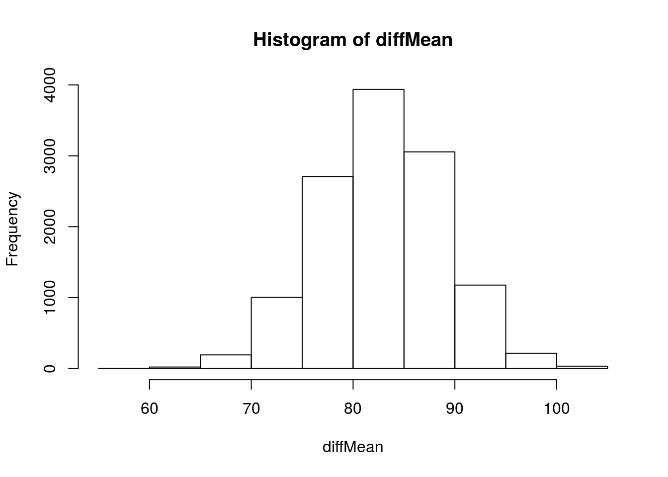
Now, let’s fit a normal curve to that (We can because we can calculate the SD directly).
# Visualize
hist(diffMean, breaks = 20, freq = FALSE)

# Add curve
curve(dnorm(x,
            mean(diffMean),
              sd(diffMean)),
      add = TRUE, col = "red3", lwd = 5)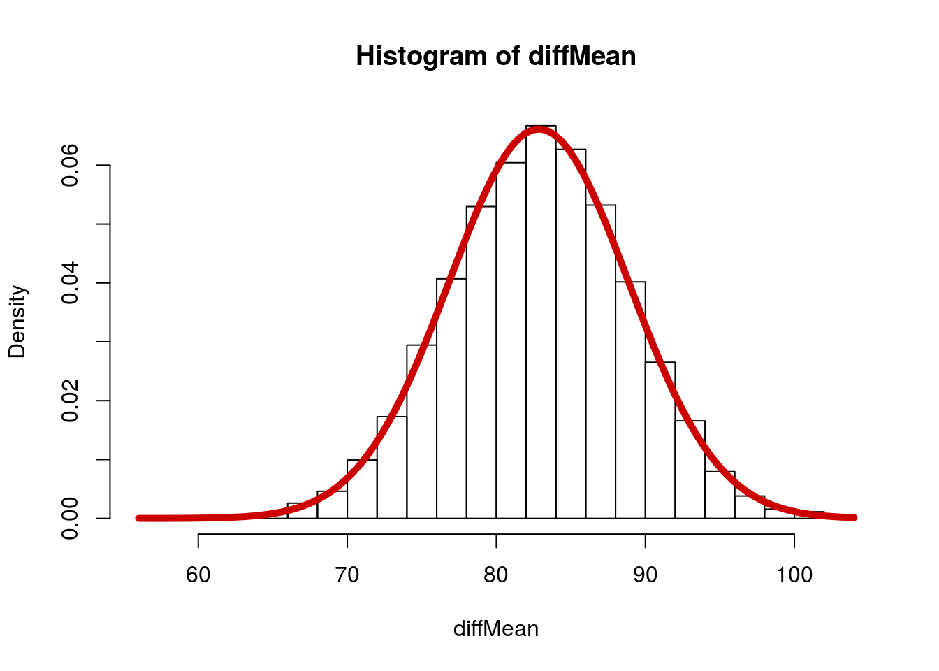
26.3.1 Estimating Standard error
So, now we just need to figure out how to estimate those values in order to use the shortcuts. The mean of the sampling distribution is simply the true population difference between the two groups, as we can see here:
# Show mean of the distribution
mean(diffMean)
## [1] 82.8515# Actual difference between groups
mean(lineWeight) - mean(skillWeight)## [1] 82.89531The standard error is a bit trickier. Luckily, however, it is very similar to the formula for the proportion. Both are, essentially:
\[ SE = \sqrt{SE_1^2 + SE_2^2} \]
Where SE1 and SE2 are the SE we would calculate for either sample alone (which makes \(SE_1^2\) \(SE_2^2\) the variance of the sampling distributions). Thus, for the difference of means, the formula is:
\[ SE = \sqrt{\frac{\sigma_1^2}{n_1} + \frac{\sigma_2^2}{n_2}} \]
where σ1 and σ2 are the two population standard deviations, and n1 and n2 are the two sample sizes. So, for the NFL data, where we have the populations sd, we can calculate it as:
\[ SE = \sqrt{\frac{\sigma_{line}^2}{n_{line}} + \frac{\sigma_{skill}^2}{n_{skill}}} \]
Which, in R, will work like this:
# Calculate the SE for differenc in means
nflSE <- sqrt( sd(lineWeight)  ^ 2 / 30 +
               sd(skillWeight) ^ 2 / 30 )
nflSE
## [1] 6.050828Which is remarkably close to our standard error based on the sampling distribution.
# Compare to calculated
sd(diffMean)
## [1] 6.029324So, we can get very, very close … if we know the population standard deviation. However, when working with the means of samples, we don’t know the population standard. So, we estimate by using the sample standard error. The formula is:
\[ SE = \sqrt{\frac{s_1^2}{n_1} + \frac{s_2^2}{n_2}} \]
Where s1 and s2 are the sample standard deviations. However, as when working with a single mean, this estimate of the standard deviation is likely to underestimate the true population standard deviation. So, we will continue to use the T-distribution when we work with means.
One other important point here is that we need to be careful about how many degrees of freedom we use for our t-distribution. We learned that for one sample, we can just use n - 1. However, for two samples, it can be a bit trickier. For this course, when calculating these by hand, we will use the smaller of the two degrees of freedom (that is, use n - 1 for whichever n is smaller). However, just bear in mind that there are more complex approaches out there[*] The formula for the degrees of freedom is technically: \[
\frac{\left( \frac{s_1^2}{n_1} + \frac{s_1^2}{n_1} \right)^2}
{ \frac{\left( \frac{s_1^2}{n_1} \right)^2}{n_1 - 1} +
\frac{\left( \frac{s_2^2}{n_2} \right)^2}{n_2 - 1}
}
\] Hopefully it is clear why I hid it here. The shortcut is close enough for now. .
26.4 Calculating a confidence interval
As we saw before for thinking about a single mean, and saw recently for the difference between two proportions, a confidence interval is just a calculated width around the point estimate from our sample. We call this width our margin of error (ME), and can calculate it with a distribution (in this case t) and our calculated SE. We use the distribution to calculate critical or threshold values (noted as t* or z* depending on the distribution) that tell us how many SE we can move away from our point estimate. Thus, multiplying t* by our SE gives us the width of our interval.
For a difference between two means, this interval is written in the form:
\[ \left(\overline{x_1} - \overline{x_2} \right) \pm ME \]
Where the two \(\bar{x}\) values are the means of the two samples. As above, the margin of error (ME) is just our t-critical value (t*) times the standard error:
\[ \left(\overline{x_1} - \overline{x_2} \right) \pm t^* \times SE \]
And, for completeness, we can right out the SE as well
\[ \left(\overline{x_1} - \overline{x_2} \right) \pm t^* \times \sqrt{\frac{s_1^2}{n_1} + \frac{s_2^2}{n_2}} \]
Let’s see this in action with some data. From the ICU data, let’s caluculate a 95% confidence interval for the difference in age between men and women.
First, let’s plot the data to see what we are working with:
plot(Age ~ Sex, data = icu)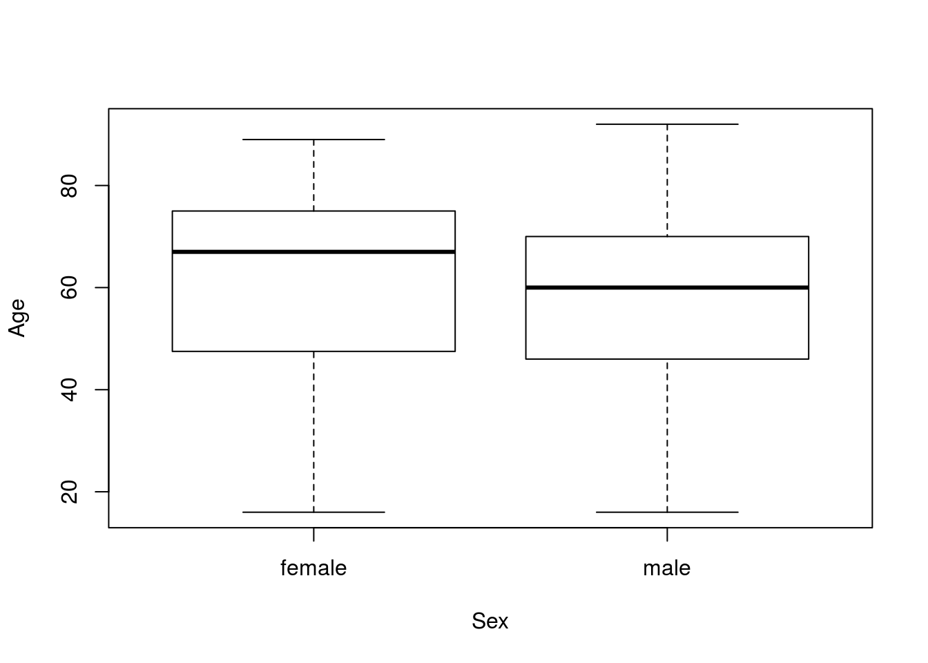
These look a bit diffent, though there seems to be a lot of overlap. Next, let’s save the values to separate variable to make our code a bit easier.
# Save variable (not always necessary)
menAge   <- icu$Age[icu$Sex == "male"]
womenAge <- icu$Age[icu$Sex == "female"]
Then, we can see how different the means are. This is our point estimate of the difference:
ptEst <- mean(menAge) - mean(womenAge)
ptEst
## [1] -3.959677So, men are -3.96 years older than women in this sample. Since we don’t usually talk about being negative years older, we might want to reverse the order of our point estimate:
ptEst <- mean(womenAge) - mean(menAge)
ptEst
## [1] 3.959677Now it is easier to say that, women are 3.96 years older than men in this sample. Next, we can calculate the standard error of the sampling distribution using the formula above. This is what we will use to decide how far we need to reach.
# Calculate SE
ageSE <- sqrt( sd(  menAge) ^ 2 / length(  menAge) +
               sd(womenAge) ^ 2 / length(womenAge) )
ageSE
## [1] 2.965941Now, we need to calculate the t-critical (t*) value to get our 95% confidence interval. This value will tell us which t-distribution to use – the smaller it is the “fatter” the tails will be to account for the fact that with small sample size we aren’t confident in our estimate of the standard deviation. For that, we first need to calculate degrees of freedom using our shortcut of one less than the smaller sample size. Here, I am using the function min(), which returns the smallest value that is passed to it (the minimum), to identify the smaller sample size.
# Calculate degrees of freedom
ageDF <- min(length(  menAge),
             length(womenAge)) - 1
ageDF
## [1] 75So, the smaller group (in this case women), had 76 samples in it. We can now calculate our t* values using qt():
# Calculate the t-critical values
tCrit <- qt( c(0.025, 0.975),
             df = ageDF)
tCrit
## [1] -1.992102 1.992102Just like for all of our other margins of error, this critical value represent the number of standard errors that we need to step away from our point estimate to capture 95% of the predicted distribution. So, we multiply by our SE to get the margin of error (using just the postive value for printing):
# Calculate margin of error
tCrit[2] * ageSE
## [1] 5.908457So, we need to reach ± 5.908 years in either direction from our point estimate to be 95% confident that we have captured the true population difference in means. We can thus report our confidence interval as a difference of 3.96 ± 5.908 years, or we can caclulate the end points:
# Calculate endpoints of CI
ptEst + tCrit * ageSE
## [1] -1.948779 9.868134In either case, we say that we are 95% confident that women patients in the ICU are between -1.949 and 9.868 years older than male patients in the ICU.
26.4.1 Try it out
Calculate a 90% confidence interval for the true population difference in the heart rate (column HeartRate) between patients in for “medical” or “surgery” visits (column Service). Make sure to plot the difference. You should get something like this:
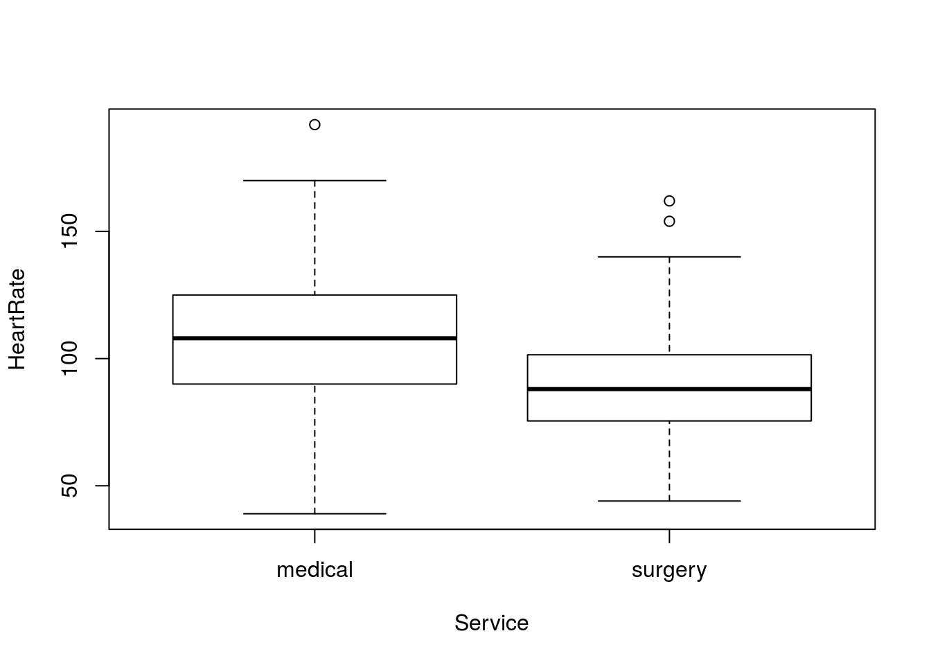
Or this:
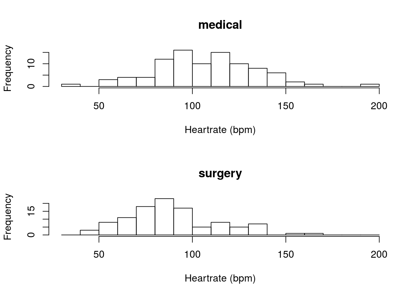
You should get a 90% confidence interval that suggests that medical patients have a heart rate that is between 11.58 and 23.63 beats per minute faster than surgery patients.
26.5 An example with given values
To complete our exercise, let’s try doing this with supplied numbers, instead of from data. In most real world applications, you will have data, but it is important that you be able to work from given values as well (particularly as the homework often supplies such values). For this, I am largely copying from above, but just replacing the calculations with given values.
Imagine that Professors A and B were evaluated by students. In this survey, Professor A got a mean score of 75 with a standard deviation of 10 from 30 students, and Professor B got a mean score of 70 with a standard deviation of 6 from 35 students. What is the 90% confidence interval for the differnce in scores between Professors A and B?
Let’s start by just entering all of the values we were given. I am going to try to use the same notations where I can so that we can copy as much code as possible.
# Professor A's info
meanA <- 75
sdA   <- 10
nA    <- 30

# Professor B's info
meanB <- 70
sdB   <- 6
nB    <- 35
Then, let’s get our point estimate, just to orient ourselves.
# Calculate difference
diffMean <- meanA - meanB
diffMean
## [1] 5Next, let’s calculate our SE. Copy the equation from above, and substitute in our known values where appropriate.
# Calculate SE
diffSE <- sqrt( sdA ^ 2 / nA +
                sdB ^ 2 / nB   )
diffSE
## [1] 2.088517Now, in one shot, we can calculate our degrees of freedom and t* values for the 90% CI.
# Calculate degrees of freedom
myDF <- min(nA, nB) - 1

# Calculate t*
qt(c(0.05,0.95), df = myDF)
## [1] -1.699127 1.699127So, we need to include values that are within 1.699 SE of our point estimate. So, we multiply by our calculated SE to get the ME then add and subtract from the point estimate to get a CI.
# Calculate ME
myME <- qt(c(0.05,0.95), df = myDF) * diffSE

# Display just the positive value
myME[2]
## [1] 3.548656# Add and subtract (use pos and neg) to get CI
diffMean + myME## [1] 1.451344 8.548656So, we are 90% confident that the true difference between the mean evaluations of Professor A and B is between 1.45 and 8.55 with the positive diffence indicating that Professor A gets better evaluations.
26.5.1 Try it out
Imagine that you sampled the mean temperature of a number of home-brewed cups of coffee and a number of cups bought at Starbucks. Given the data below, calculate a 99% confidence interval for the true difference in temperature.
| Starbucks | Home | |
|---|---|---|
| mean | 180 | 175 |
| sd | 2 | 3 |
| n | 8 | 10 |
You should get a confidence interval of 0.859 and 9.141 degrees.