An introduction to statistics in R
A series of tutorials by Mark Peterson for working in R
Chapter Navigation
- Basics of Data in R
- Plotting and evaluating one categorical variable
- Plotting and evaluating two categorical variables
- Analyzing shape and center of one quantitative variable
- Analyzing the spread of one quantitative variable
- Relationships between quantitative and categorical data
- Relationships between two quantitative variables
- Final Thoughts on linear regression
- A bit off topic - functions, grep, and colors
- Sampling and Loops
- Confidence Intervals
- Bootstrapping
- More on Bootstrapping
- Hypothesis testing and p-values
- Differences in proportions and statistical thresholds
- Hypothesis testing for means
- Final thoughts on hypothesis testing
- Approximating with a distribution model
- Using the normal model in practice
- Approximating for a single proportion
- Null distribution for a single proportion and limitations
- Approximating for a single mean
- CI and hypothesis tests for a single mean
- Approximating a difference in proportions
- Hypothesis test for a difference in proportions
- Difference in means
- Difference in means - Hypothesis testing and paired differences
- Shortcuts
- Testing categorical variables with Chi-sqare
- Testing proportions in groups
- Comparing the means of many groups
- Linear Regression
- Multiple Regression
- Basic Probability
- Random variables
- Conditional Probability
- Bayesian Analysis
Using the normal model in practice
19.1 Load today’s data
Start by loading today’s data. If you need to download the data, you can do so from these links, Save each to your data directory, and you should be set.
- Roller_coasters.csv
- Data on the height and drop of a sample of roller coasters.
- icuAdmissions.csv
- Data on patients admitted to the ICU.
# Set working directory
# Note: copy the path from your old script to match your directories
setwd("~/path/to/class/scripts")

# Load data
rollerCoaster <- read.csv("../data/Roller_coasters.csv")
icu           <- read.csv("../data/icuAdmissions.csv")
19.2 Overview
Now that we can draw and make normal plots … so what? How can we use them? In this chapter, we will look at some of the properties of the normal model and how we can use them to approximate confidence intervals and p-values. Here, we will compare them directly to the results from our previous approaches to show that they give similar answers.
19.3 Estimating Confidence Intervals
We’ve already encountered the normal model when working with Confidence Intervals (CI’s). When we used the 95% rule (that 95% of values are within 2 Standard errors of the mean), we were implicitly using the normal approximation. Now, instead of using that one approximation, we can calculate any confidence interval we want.
To start, we will again use the roller coaster bootstrap sample. This is copied from last chapter:
# Coaster bootstrapping

# Initialize vector
coasterBoot <- numeric()

# Loop through many times
for(i in 1:12489){
  # calculate the correlation
  # note, we could save these each as a vector first
  # but we don't need to
  coasterBoot[i] <- mean(sample(rollerCoaster$Speed,
                                replace = TRUE)
                         )
}

# Plot the result
hist(coasterBoot,
     freq = FALSE,
     breaks = 60,
     main = "Bootstrap of Coaster Speed",
     xlab = "Mean Speed (mph) in sample")

# Plot the coaster bootstrap distribution
# Add a curve to the plot
curve(dnorm(x,
            mean = mean(coasterBoot),
            sd   =   sd(coasterBoot)),
      col = "purple", lwd=3,
      add = TRUE)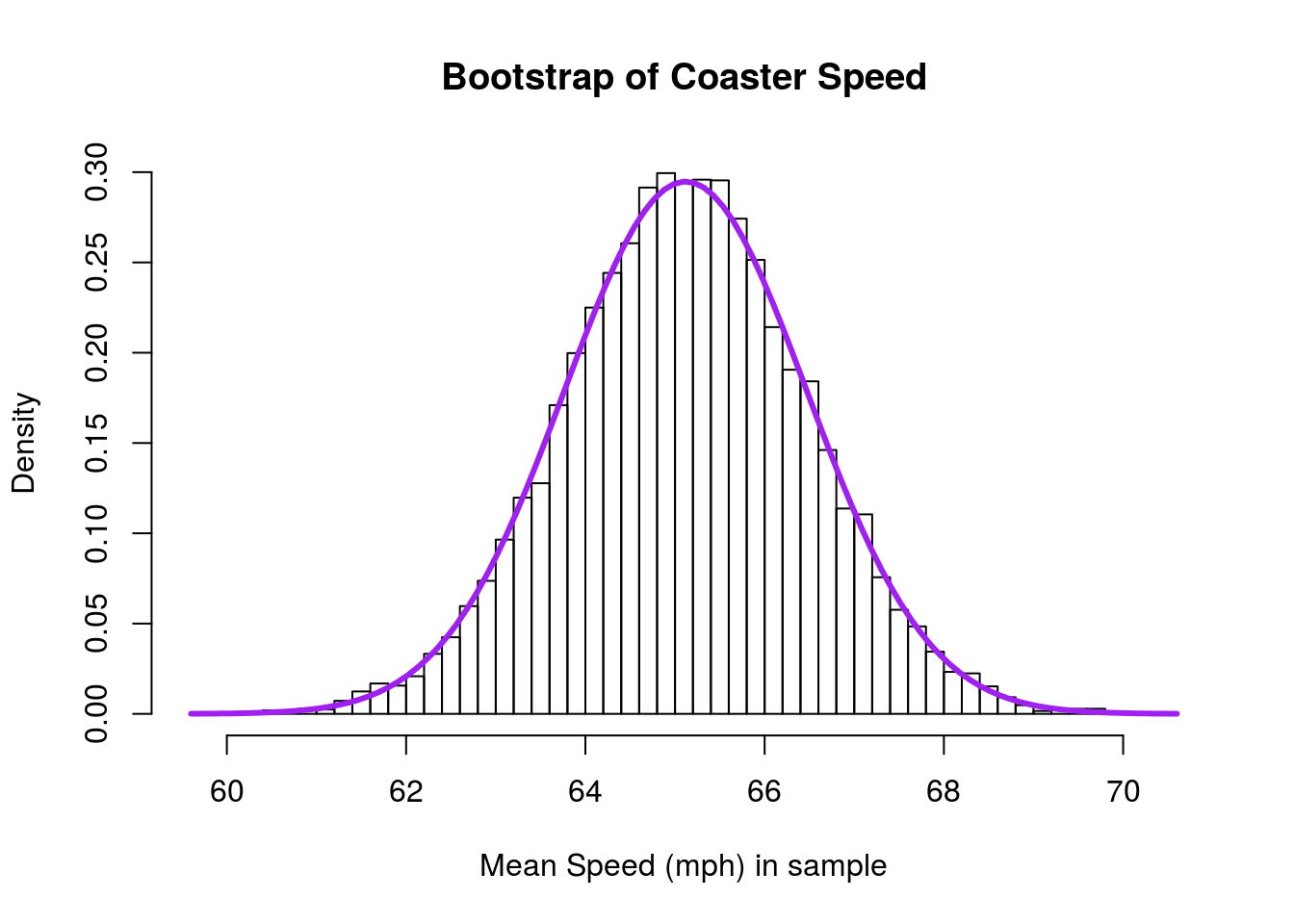
To calculate a 95% confidence interval, we have been using quantile():
# Calculate 95% CI
quantile(coasterBoot, c(0.025,0.975))
## 2.5% 97.5%
## 62.4608 67.7848Telling us that we are 95% confident that the true population mean lies between 62.46 and 67.78 mph. We can also use the normal curve directly to calculate this. The mechanics are the same, the only difference is that instead of giving the function the whole distribution, we only need to specify the mean and sd. For this, we use the function qnorm(), which gives us the quantiles of the normal distribution.
# Calculate a 95% CI
qnorm(c(0.025, 0.975),
      mean = mean(coasterBoot),
      sd   =   sd(coasterBoot))
## [1] 62.4653 67.7694Note that these values are remarkably close to those we calculated with quantile(). Further, just like with quantile(), we can change the cutoffs to get different CI’s.
# Calculate a 90% CI
qnorm(c(0.05, 0.95),
      mean = mean(coasterBoot),
      sd   =   sd(coasterBoot))
## [1] 62.89168 67.34302# Calculate a 99% CI
qnorm(c(0.005, 0.995),
mean = mean(coasterBoot),
sd = sd(coasterBoot))## [1] 61.63196 68.6027419.3.1 Visualizing normal cutoffs
It is helpful to remember what it is we are looking at. So, let’s add vertical lines for the 95% CI to our plot
# Add 95% CI lines
abline(v = qnorm(c(0.025, 0.975),
                 mean = mean(coasterBoot),
                 sd   =   sd(coasterBoot)),
       col = "darkblue",
       lwd = 3, lty = 3)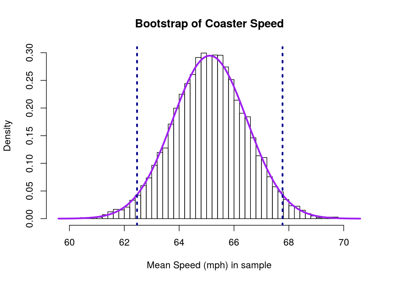
When using quantile() before, we were interested in what proportion of the data fell outside those thresholds (set as 2.5% on each side). When using the normal model, we are asking the same question, but with a twist. We are now interested in what proportion of the area under the curve is outside of those thresholds (again, set as 2.5% here).
This may seem like semantics, but it will matter soon. The goal we are driving towards is to be able to use the normal model without having to rely on the computationally intensive loops we’ve been using.
19.3.2 Try it out
Copy one the bootstrap distribution you made in the previous chapter. Draw the normal curve on it, then calculate a 90% CI using each quantile() and qnorm(). Add lines to the plot representing the cut off.
19.4 Estimate p-values with the normal model
Let’s start by addressing a question from an earlier chapter: Are male and female ICU patients the same age?
As always, we need to think about what this question means, and write out our hypotheses. As is (almost) always the case, the most boring thing that could be true is that the two groups have the same mean age. Our alternative, in this case, will be that they are not the same mean age.
H0: mean age of men is equal to the mean age of women
Ha: mean age of men is not equal to the mean age of women
Now that we have hypotheses in mind, let’s take a look at the data. It is always good to start with a picture:
plot(Age ~ Sex, data = icu)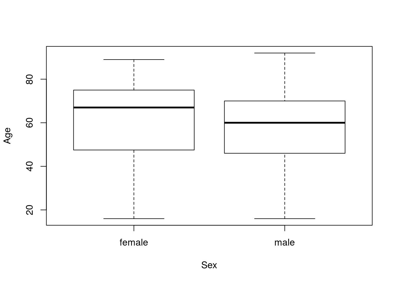
As before, there is some difference in the ages, but not a lot. So, we can then create a null distribution. This is all copied from an earlier chapter.
# Calculate the means
ageMeans <- by(icu$Age, icu$Sex, mean)

# Calculate the difference
ageDiff <- ageMeans["male"] - ageMeans["female"]

# Initialize variable
nullAgeDiff <- numeric()

for(i in 1:17654){
  # draw a randomized sample of ages
  tempAges <- sample(icu$Age,
                     size =  nrow(icu),
                     replace = TRUE)

  # calculate the means
  tempMeans <- by(tempAges, icu$Sex, mean)

  # Store the parameter of interest (the difference in means here)
  nullAgeDiff[i] <- tempMeans["male"] - tempMeans["female"]
}

# Visualize
hist(nullAgeDiff,
     main = "Null distribution of age difference by sex",
     xlab = "Sample difference in age (male - female)")
# Add lines for our data
abline(v = c(ageDiff, - ageDiff),
       col = "green3",
       lwd = 3, lty = 3)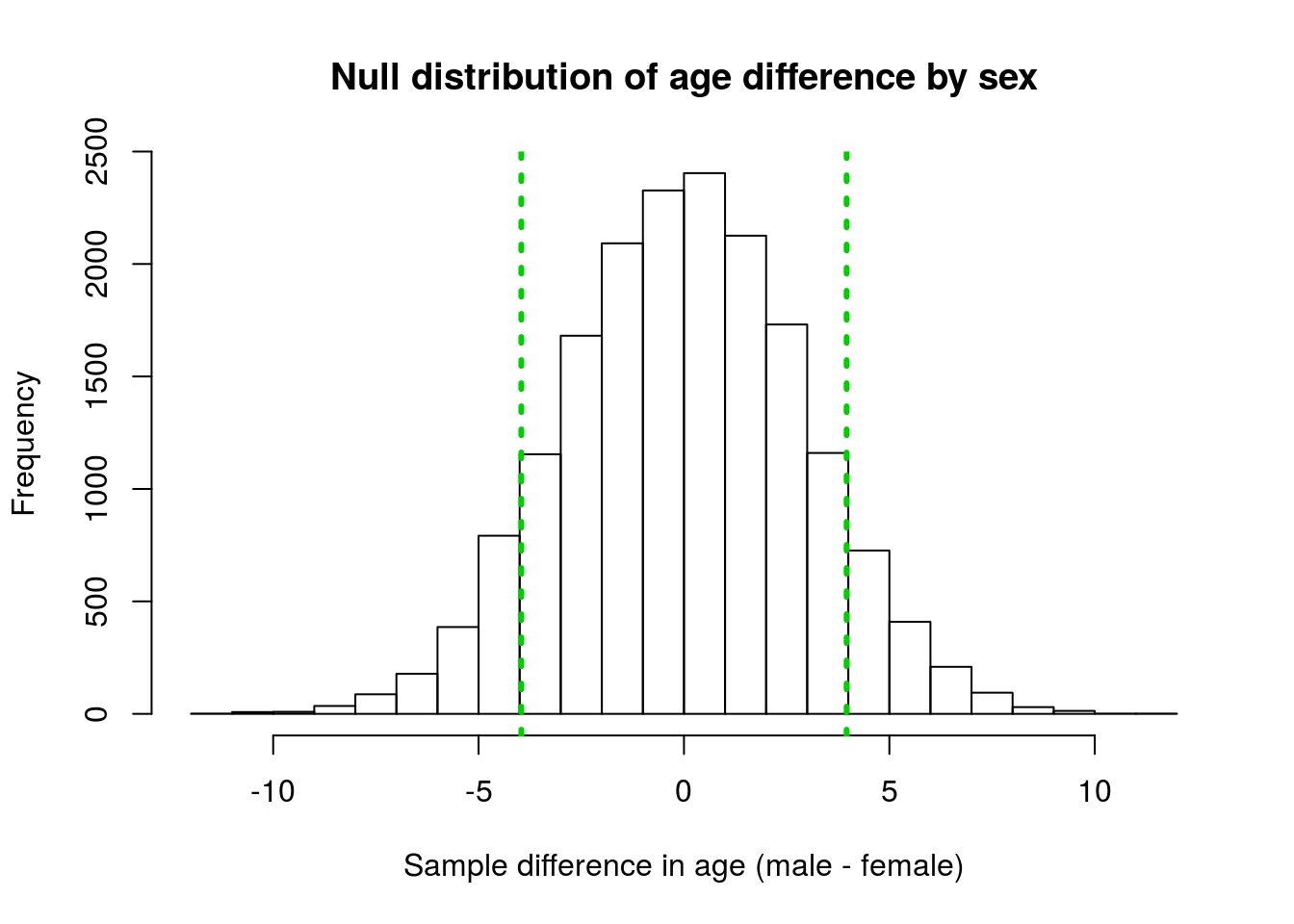
We calculated the p-value as the area outside of those vertical lines because those are the points from the null distribution that are as extreme as, or more extreme than, our observed data. Below is the code copied from that previous use:
# Safer p-value calculation
pVal <- mean(nullAgeDiff >=  abs(ageDiff) |
             nullAgeDiff <= -abs(ageDiff)  )
pVal
## [1] 0.1732185This p-value was large enough that we did not reject the H0, so cannot say that there is a difference in age between the two sexes.
Now, let’s apply the normal model to this case. Start by adding the normal curve to the plot. Note that we need to change the histogram to density, and I think it looks better with a few more breaks. Feel free to play with any of these parameters to make a nice looking plot.
One point worth remembering is that, because we have set our H0, we always use that as our mean, rather than the mean of the distribution (which can vary a bit due to sampling differences)
# Visualize
hist(nullAgeDiff,
     main = "Null distribution of age difference by sex",
     xlab = "Sample difference in age (male - female)",
     freq = FALSE,
     breaks = 20)
# Add lines for our data
abline(v = c(ageDiff, - ageDiff),
       col = "green3",
       lwd = 3, lty = 3)

# Add the normal curve
curve(dnorm(x,
            mean = 0,
            sd   = sd(nullAgeDiff)),
      add = TRUE,
      col = "red3", lwd = 3)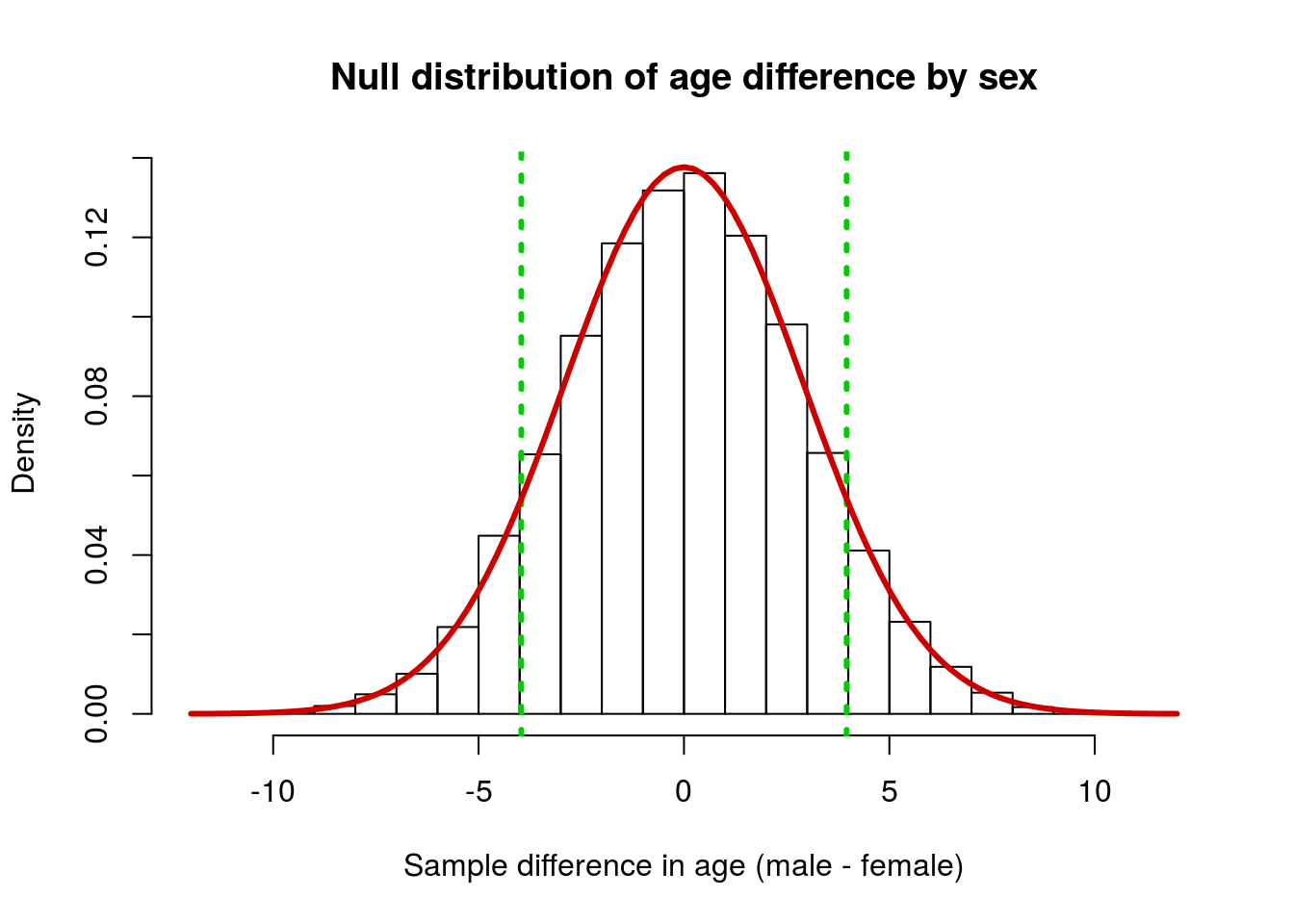
To calculate the area under the curve to the left of a point, we use the function pnorm(). The concept is similar to how we calculated the p-value above: we are asking what proportion of the area is to the left of the point we ask about. Because the function always gives the area to the left, it is often easier to start with the lower limit from the plot.
# Calculate area below left cut off
pnorm(-abs(ageDiff),
      mean = 0,
      sd   = sd(nullAgeDiff))
## male
## 0.08584861Note that I am using -abs() to make sure that I have the left hand side. However, this is only counting one tail of the distribution, and our Ha was two tailed.
So, we also need to calculate the area to the right of the right hand line. Because pnorm() by default returns the area to the left of a point, we need to be a little bit careful. Luckily, however, by using the density, the area under the entire curve is always exactly 1. Therefore, we can just subtract the area to the left from one, and we will get the area to the right.
# Calculate area above right cutoff
1 - pnorm(abs(ageDiff),
          mean = 0,
          sd   =   sd(nullAgeDiff))
## male
## 0.08584861You probably notice that this value is exactly the same as the area below the left threshold. Because the normal model is, by definition, perfectly symmetrical, we can simply double the value of one tail to get our two tailed distribution.
# Calculate the two tailed p-value
2 * pnorm(-abs(ageDiff),
          mean = 0,
          sd   =   sd(nullAgeDiff))
## male
## 0.1716972Giving us almost exactly the same p-value as we calcluated from the distribution directly (0.1732).
19.4.1 A note on areas
The above subtraction works for other intervals as well. To get the area between two points, first calculate the area to the left of each. Because the area between them is just the difference you can subtract the area of the lower number from the area of the bigger number. For example, to get the area between the two lines we can calculute:
# Calculate area below left line
areaBelowLeft  <- pnorm(-abs(ageDiff),
                        mean = 0,
                        sd   =   sd(nullAgeDiff))
# Calculate area below right line
areaBelowRight <- pnorm(abs(ageDiff),
                        mean = 0,
                        sd   =   sd(nullAgeDiff))
# Calculate the difference
areaBelowRight - areaBelowLeft
## male
## 0.8283028This tells us that 82.83% of the distribution is less extreme than our observed data. Notice that this is the same as 1 - pVal, since the whole area has to sum up to 1.
This type of calculation is less applicable to this kind of distribution, but it is helpful to understand this property of distribution densities.
19.4.2 Try it out
Go back to an earlier script and copy another hypothesis test question that we calculated. Paste in the code to generate the null and calculate the p-value. Then, visualize the distribution and add the normal curve on top of it. Calculate the p-value using pnorm() and compare it to the value you got with the old method.
19.5 Scaling data
Earlier, I mentioned that R uses the “standard” normal as a default, without talking much about it. The standard normal is simply a normal distribution that is centered at 0 with a standard deviation of 1. In addition to being a common default, it provides a useful yardstick to compare things on different scales, using the z score that we learned about earlier this semester. Recall that the z score was centered at 0 with a standard deviation of 1. (This is not an accident.)
We can, thus, convert our data to z-scores and plot it to utilize the standard normal model. Until recently, this was incredibly important as it allowed a single table of printed quantiles for the normal distribution to be used for any distribution. With the rise of technology, it is no longer very hard to calculate quantiles for any normal distribution, but it is still useful for standardization and to understand the calculations in some of the tests we will see soon.
A note here: Many other texts and problem sets ask/recommend you to convert to z-scores for a lot of things. I tend to find it more confusing, and prefer to pass the mean/sd to whatever function I need (e.g pnorm, dnorm, and qnorm). However, either approach will yeild the same answers. Later this semester we will see some cases where we do need to convert to z-scores, so it is helpful to consider now.
Recall that the z score of a value can be calculated as:
\[ z_i = \frac{x_i - \bar{x}}{\sigma_x} \]
Where x is a numeric variable, i represents the index (so \(x_i\) is the ith value of x), \(\bar{x}\) is the mean of x, and \(\sigma_x\) is the standard deviation of x. In R, we can calculate this as:
z <- (x - mean(x) ) / sd(x)Where x is a vector (so each value is used of “x” and the single sample value is used for the mean and sd).
Doing this for the coaster data, we get:
# Scale coaster data
scaledCoaster <- (coasterBoot - mean(coasterBoot) ) /
                    sd(coasterBoot)
We can then plot it and overlay the standard normal curve by not specifying a mean or standard deviation
# Plot it
hist(scaledCoaster,
     breaks = 20,
     xlab = "Scaled Speed (z-score)",
     freq = FALSE)

# Add the standard normal line
curve(dnorm(x),
      add = TRUE,
      col = "purple",
      lwd =3)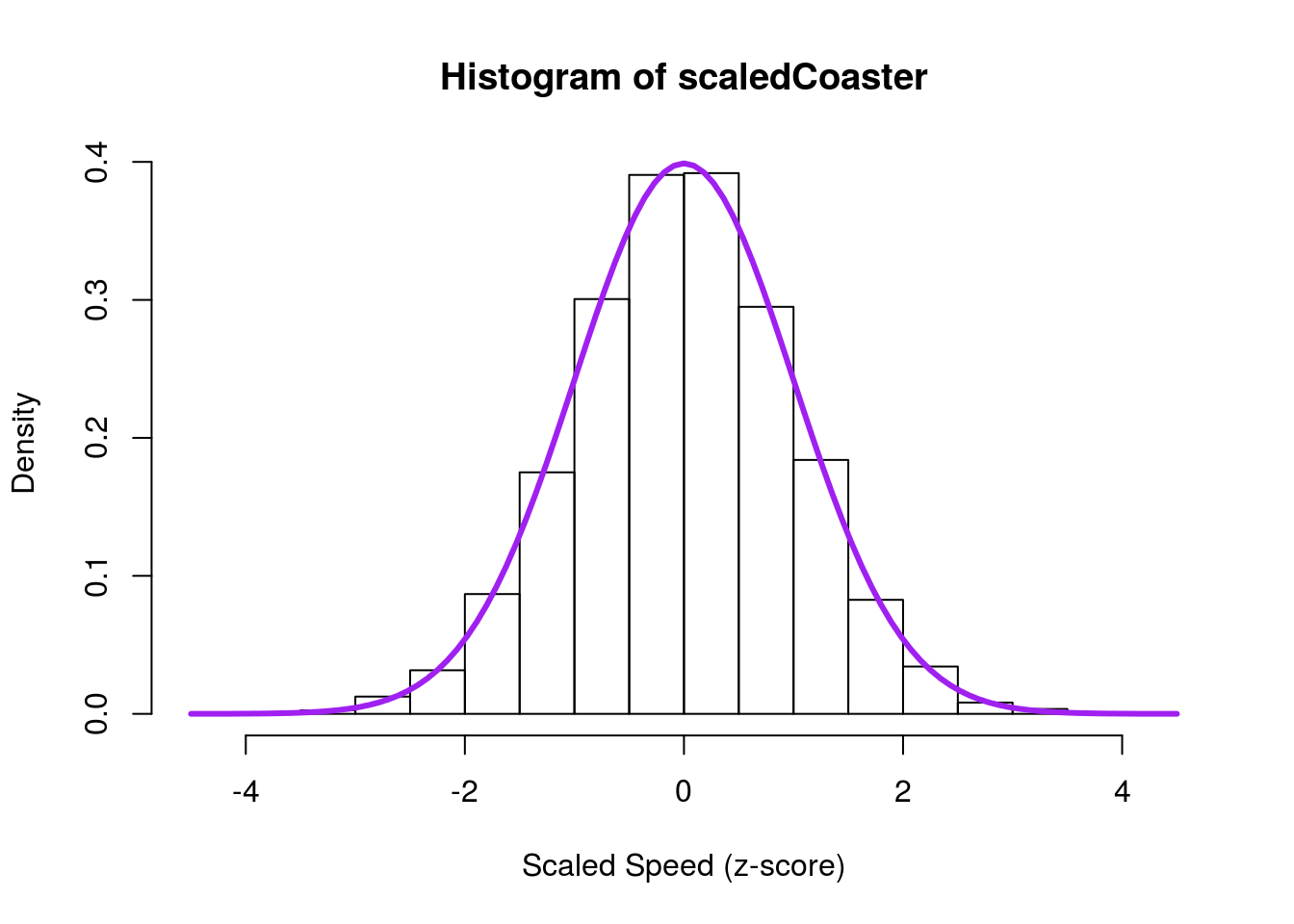
Note that the histogram looks nearly identical to what it did before, but is now centered at 0 with a standard deviation of 1. We can see this more clearly by plotting the values against each other.
# Plot scale vs. unscaled
plot(scaledCoaster ~ coasterBoot)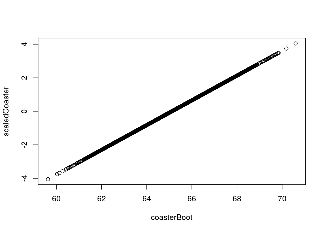
19.6 Central limit theorem
The central limit theory is what allows us to use a normal approximation. It’s definition is something, for now, you have to trust, though we will work through some of it’s details over the next few weeks. It’s definition:
Central limit theorem
For sufficiently large sample sizes, the means (or proportions) from multiple samples will be approximately normally distributed and centered at the value of the population parameter (e.g. mean or proportion).
This means that, for our bootstrap and null distributions, as long as the sample size is sufficiently large, we can treat the distribution as if it is normal (which we’ve seen above). The precise definition of sufficiently large and the standard deviation will be discussed more as we encounter cases where they are needed. This chapter justifies (by demonstration) our use of normal approximations in the scenarios that will come in the chapters that follow.
Thus, we can use the pnorm function to find confidence intervals and p values instead of calculating them directly from the quantiles of our distributions (null or bootstrap).
This should give us very similar answers, and for the moment doesn’t change much of what we are able to do or infer. However, the normal model approach only requires two inputs: the mean and the standard deviation. We know that the mean of our bootstrap value should be near the point estimate of our original sample, and the mean of our null is defined by H0. In the coming chapters, we will use approximations for the standard deviation to allow us to avoid bootstrapping and null distributions altogether.
This shortcut was far more important in the past, when, without computers (and R) it was difficult to collect boostrap and null samples. Despite moving past this limit, these shortcuts (and the tests they spawned) are still commonly used, and provide us more direct answers to questions.
By building through bootstrap and null sampling, hopefully you have developed an intuition for interpretting these values. In addition, the field of statistics appears to be slowly moving away from reliance on these “normal” shortcuts.