An introduction to statistics in R
A series of tutorials by Mark Peterson for working in R
Chapter Navigation
- Basics of Data in R
- Plotting and evaluating one categorical variable
- Plotting and evaluating two categorical variables
- Analyzing shape and center of one quantitative variable
- Analyzing the spread of one quantitative variable
- Relationships between quantitative and categorical data
- Relationships between two quantitative variables
- Final Thoughts on linear regression
- A bit off topic - functions, grep, and colors
- Sampling and Loops
- Confidence Intervals
- Bootstrapping
- More on Bootstrapping
- Hypothesis testing and p-values
- Differences in proportions and statistical thresholds
- Hypothesis testing for means
- Final thoughts on hypothesis testing
- Approximating with a distribution model
- Using the normal model in practice
- Approximating for a single proportion
- Null distribution for a single proportion and limitations
- Approximating for a single mean
- CI and hypothesis tests for a single mean
- Approximating a difference in proportions
- Hypothesis test for a difference in proportions
- Difference in means
- Difference in means - Hypothesis testing and paired differences
- Shortcuts
- Testing categorical variables with Chi-sqare
- Testing proportions in groups
- Comparing the means of many groups
- Linear Regression
- Multiple Regression
- Basic Probability
- Random variables
- Conditional Probability
- Bayesian Analysis
Bootstrapping
12.1 Load today’s data
Start by loading today’s data. If you need to download the data, you can do so from these links, Save each to your data directory, and you should be set.
- NFLcombineData.csv
- Data on the Height, Weight, and position type of all 4299 players that participated in the NFL combine during the collection period
- mlbCensus2014.csv
- Basic data on every Major League Baseball player on a 25-man roster as of 2014/May/15
# Set working directory
# Note: copy the path from your old script to match your directories
setwd("~/path/to/class/scripts")

# Load data
nflCombine <- read.csv("../data/NFLcombineData.csv")
mlb        <- read.csv("../data/mlbCensus2014.csv")
12.2 A note on sample statistics
For all of the things we have done so far, and will do in this chapter, we could measure any sample statistic that we wanted to. We have done means and proportions, but if we were interested in some other population parameter, such as the standard deviation or the median, we could just as easily calculate that from our samples. Don’t get caught in a trap of thinking that the metrics we are showing are the only possible ones.
Do be aware, however, that some metrics are not well suited to these methods. For example, while the median is possible to evaluate, calculating it from a small sample (especially with the methods introduced in this chapter) is not always ideal. Always plot the results of any simulation (usually a histogram, as we have been doing). Most common problems can be identified quickly by following that simple step.
12.3 Estimating standard errors
So far, we have collected many, many samples, calculated a statistic from them, and then calculated the standard deviation (which in this special case is called the standard error). How often, in the real world, can you collect 1000 sample to determine the standard error? Almost never!
In reality, we need to estimate the standard error, and that is where we are going in this chapter. Instead of sampling many times, we will sample once and then simulate sampling multiple times.
12.4 A physical example
Imagine a cup full of red and white pony beads.

If you wanted to calculate the proportion that are red (the population parameter), what would you do? You would likely count all of the beads, then divide the number of red by the total number.
What if, however, the cup was exceedingly large (for example, a mixing vat at the factory), and you didn’t have a way to count all of the beads? How might we estimate the proportion?
We would probably draw a smaller sample of beads, then calculate the proportion of those that are red. That is exactly what an introductory statistics course did. Let’s enter the numbers they drew below.
Note the use of the new command rep(). This function can be used in a number of ways (and we will see several of them). One of the simplest uses is seen here: it tells the computer to repeat each of the values in the first argument the number of times in the second argument. Note that if the two arguments are different lengths, very different things can happen (they are usually good and what we want, just not here).
# Enter the data from the class sample
classBeadSample <- rep(c("red", "white"),
                       c(  10 ,   5   ) )
# Display the data
table(classBeadSample)
## classBeadSample
## red white
## 10 5From this we can estimate the proportion of beads as follows
# Save and display the calculated values
propRedSample <- mean(classBeadSample == "red")
propRedSample
## [1] 0.6666667But, how much confidence should we have in the estimate? Previously, we would have sample many times, calculated the standard deviation of the statistic (here, proportion that are red), and called that our standard error.
But, what if such samples are too difficult? For example, what if it was expensive to collect the beads? For that, we will introduce bootstrapping.
12.5 Bootstrapping
The term “bootstrapping” is derived from the colloquial phrase “pull yourself up by your bootstraps,” which generally means working from whatever little you have to improe your lot. We are going to do the same thing by using our small sample to estimate how confident we should be in our estimate.
The general idea is to simulate taking multiple samples, assuming that our initial sample is a generally good representation. That may seem like a big assumption, but it is a relatively safe one. First, it is unlikely for any one sample to be exceedingly weird. It is possible, but unlikely. Second, and this is more important for means than proportions, we expect the general shape of the distribution to be similar. Thus, even if the estimated statistic (e.g. proportion or mean) is off by a bit, the shape will still give us enough information to draw conclusions. Finally, sometimes the sample won’t be a very good representation, but those are the times when we are wrong – and that is ok. Just as we saw before, when we set a 95% confidence level, about 5% of the time the confidence interval will not contain the true value, and that is to be expected.
The process of bootstrapping is straightforward. We treat our sample as if it is truly representative of the population, then draw a number of samples from that new simulated population. There are two key components to this sampling: the sample size must remain the same as our original sample, and the sampling must be done “with replacement” (defined in a moment).
As we saw with sampling distributions, the sample size plays a major role in our confidence that we are accurately estimating the population parameter. So, we cannot change the sample size or our results won’t be meaningful.
If we are keeping the same sample size, then every sample would be the same if we just drew each bead once. By drawing “with replacement”, we ensure that we can get different values each time. More philosophically, sampling with replacement is equivalent to making our population infinitely large with the proportion of red beads set to be the value we calculated in our sample.
To do this physically, we would draw a bead out of our initial sample, record its color, then return it to the cup before drawing again. For each bootstrap sample, we then calculate our statistic (here, proportion that are red).
Here are the results of a few from the intro stats course:
# Initialize our vector to hold statistics
inClassBootStats <- numeric()

# Record first sample
tempBootSample <- rep(c("red", "white"),
                      c(   9 ,   6   ) )

# Store the value in the first slot
inClassBootStats[1] <- mean(tempBootSample == "red")

# record additional samples
tempBootSample <- rep(c("red", "white"),
                      c(   11 ,   4   ) )

# Store the value in the next slot
inClassBootStats[2] <- mean(tempBootSample == "red")

# record additional samples
tempBootSample <- rep(c("red", "white"),
                      c(   10,   5   ) )

# Store the value in the next slot
inClassBootStats[3] <- mean(tempBootSample == "red")
We could collect more, but for the moment, let’s just see what we have.
# Visualize in class boot strap samples
hist(inClassBootStats)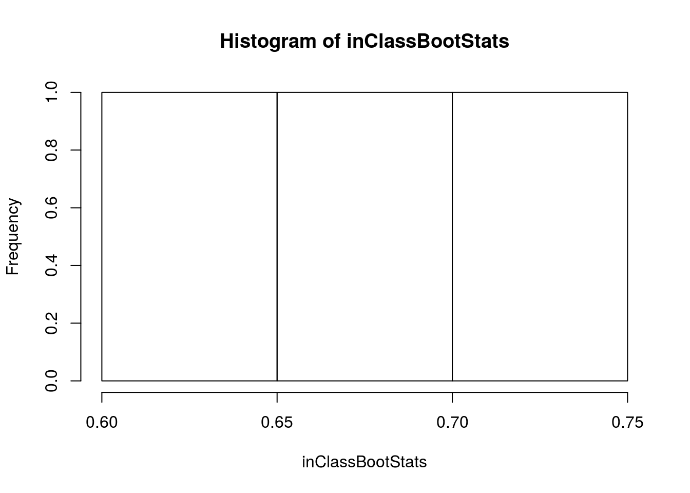
Here, we could use the standard deviation of our bootstrap distribution to estimate our standard error. However, to do so accurately, we would need to collect many more bootstrap samples. Instead of spending the next week collectin these samples by hand, lets try using R instead.
12.6 Using R to simulate bootstraps
You may have noticed that the above code looks very similar to something else we have encountered in R before. Instead of copy-pasting the sampling many times (and having to remember to change the index), we can instead use a for() loop. The below was copied from our manual bootstraps above then wrapped in a for loop. I replaced our manual sample with the sample() command and added the i for the index instead of the separate values. Notice that we have added the argument replace = TRUE to the sample() function. This argument is what ensures that our sample is taken with replacement.
# View our sample, just as a reminder
table(classBeadSample)
## classBeadSample
## red white
## 10 5# Initialize our variable (we can use the same one we used above)
# This will erase the values that were in it
inClassBootStats <- numeric()
# Loop an arbitrarily large number of times
# More will give you a more accurate and consistent distribution
for(i in 1:8793){
# collect a sample
tempBootSample <- sample(classBeadSample,
size = length(classBeadSample),
replace = TRUE) # NOTE: we need this line
# Store the value in the first slot
inClassBootStats[i] <- mean(tempBootSample == "red")
}Now, we can look at the distribution and calculate our standard error:
# Visualize more samples
hist(inClassBootStats)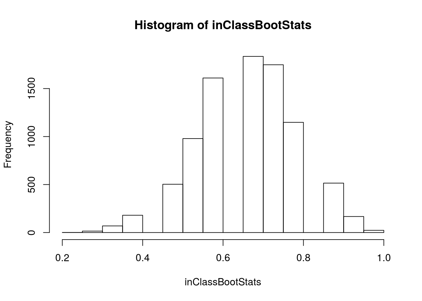
# Calculate standard errof
sd(inClassBootStats)
## [1] 0.1220486Here, we can say that our standard error is about 0.12. Recall that we our 95% confidence interval is plus or minus two standard errors, so we are 95% confident that the true population value falls between 0.42 and 0.91. We can also mark this interval on our histogram, to help us visualize.
# Add lines
abline(v = propRedSample + c(-2,2)*sd(inClassBootStats),
       col = "green3", lwd = 3, lty = 2)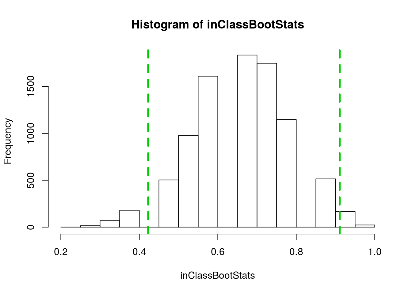
Remember that we cannot know for sure if our confidence interval captures the true value most of the time when we calculate such and interval. However, we do believe that about 95% of the time that we construct a 95% confidence interval, it will capture the true population parameter.
12.6.1 Try it out
We can use these same tools on data that we have in the computer. Let’s imagine that we want to know what proportion of MLB players are pitchers (and that we didn’t have the whole census). Take a sample from the POS.Broad column of the mlb data using the code below. Note that your sample will (almost certainly) be different than mine.
# Take a sample of positions
posSample <- sample(mlb$POS.Broad,
                    size = 55)
# Look at the result
table(posSample)| Catcher | Designated Hitter | Infielder | Outfielder | Pitcher |
|---|---|---|---|---|
| 3 | 0 | 15 | 14 | 23 |
And you can see your estimated proportion with:
# Sample proportion
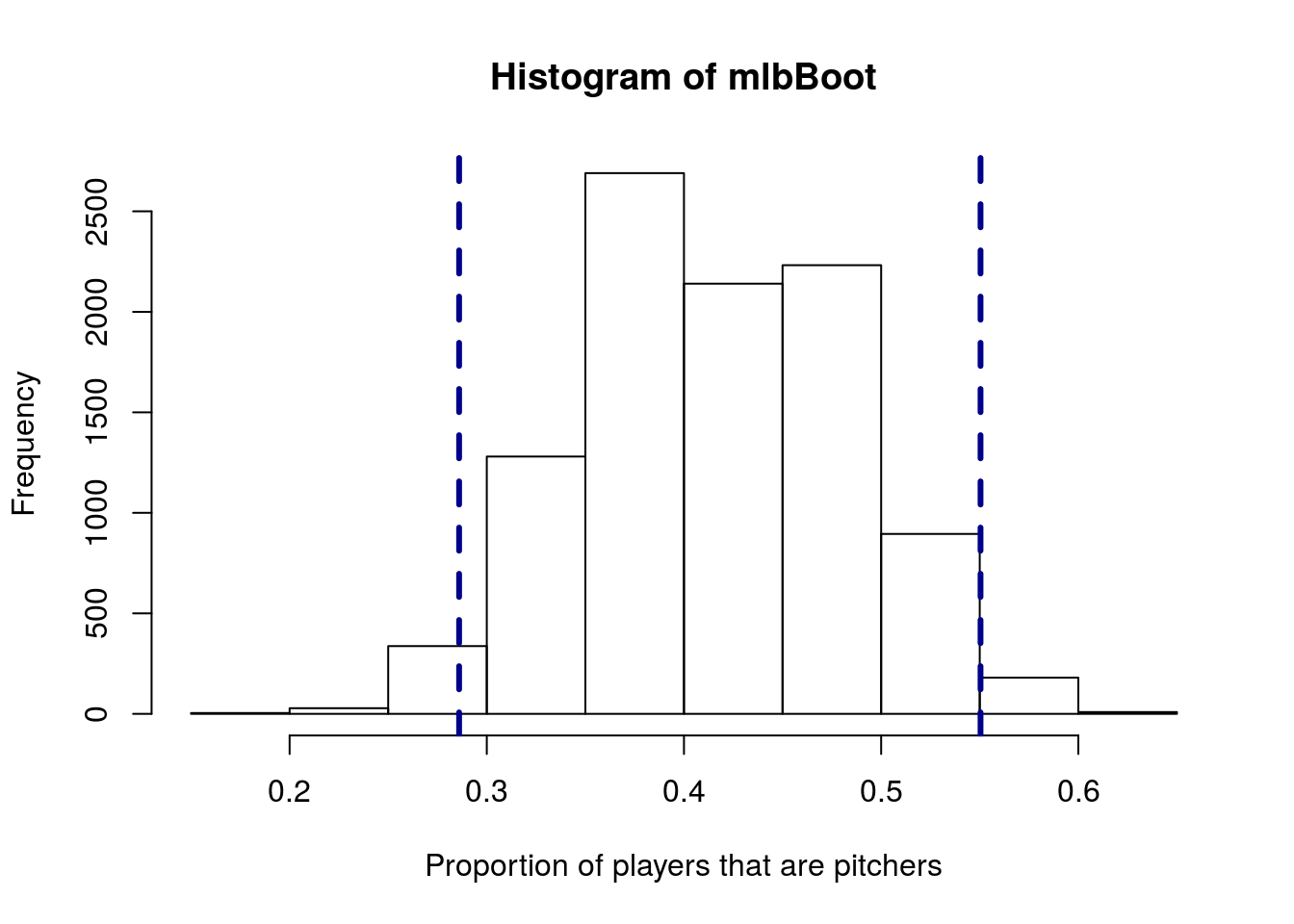
mean(posSample == "Pitcher")## [1] 0.4181818Then, use bootstrap sampling to estimate the standard error and 95% confidence interval. You should get something like this:
12.7 Compare to our previous method
Now, it is time to reveal that the true proportion of beads that are red is 0.50. Is that within our calcultated 95% confidence interval?
Knowing that information, lets take multiple samples in order to compare our bootstrap result to an empirical result. Recall that we are only interested, for this purpose, in calculating the standard error.
# create a vector of the full population
beadPopulation <- rep(c("red","white"),
                      c( 100 ,  100  )  )
table(beadPopulation)
## beadPopulation
## red white
## 100 100Now, we can collect multiple samples and calculate the standard error.
# Initialize vector
beadSampleProp <- numeric()

# Loop for multiple samples
for(i in 1:9016){
  # Take a sample
  tempBeadSample <- sample(beadPopulation,
                           size = length(classBeadSample))

  # Store the proportion
  beadSampleProp[i] <- mean(tempBeadSample == "red")
}

# Calculate the standard error
sd(beadSampleProp)
## [1] 0.1239263Is that standard error similar to our bootstrap? It should be, and that is why this works. The calculated standard error from the example above was 0.122, which is quite close to the 0.124 that we calculated here.
This does not mean that the in class sample was (necessarily) a good one or that the true value was within our confidence interval. But, it does show us that the standard deviation of a bootstrap sample is a reasonable approximation of the standard error. This allows us to give confidence intervals without having to know the full population (which would defeat the purpose).
12.7.1 Try it out
Create a new sampling distribution to estimate the standard error the of the proportion of MLB players that are pitchers. That is, create many samples from the full population, and calculate the standard error. The value should be relatively close to the estimate you got from the bootstrap above. If it is not – check to make sure that your sample sizes are correct.
12.8 An example with means
Now that we have the mechanics mostly worked out, let’s look at an example more similar to what we might encounter in the real world. We could replace “beads” with people (and color with gender) or use survival of a disease (with color now representing living or dying). Instead, let’s remind ourselves that this works on a broad range of statistics, and estimate mean weight of NFL combine participants again.
First, let’s take a sample of NFL weights. This might be what we could do if we were only able to sample a small number of participants. Here, I am also going to introduce the function set.seed(), which is a tool that allows you to get repeatable results. The random generators in R (and all other computers) use a “seed” from which to start their processes[*] It is in this sense that random generators on computers are actually pseudo-random. They are deterministic but give patterns similar to random chance. Usually, they arbitrarily pick a seed (based on something like the time when you start it), which is why you usually get different results when running the same command. .
By setting this seed, you can get the same results out every time you run the same command. Here, it is useful so that you start with the same sample as is given, but it can also be very useful in homeworks or exams so that the values generated by your sampling or bootstrap loops are the same in the html output as they are when you run it on the computer.
# Set seed for consistent results
# Don't always use the same one
set.seed(230)

# take a sample
nflSamples <- sample(nflCombine$Weight,
                     size = 40)

# Look at the sample mean
mean(nflSamples)
## [1] 259.275But, this doesn’t tell us how confident we should be. For that, we need to bootstrap a sample distribution, then calculate the standard error. Try it.
# Initialize vector
nflBoot <- numeric()

# Loop through the sample
for(i in 1:12489){
  # take a bootstrap sample
  tempNFLboot <- sample(nflSamples,
                        size = length(nflSamples),
                        replace = TRUE)
  # Save the mean
  nflBoot[i] <- mean(tempNFLboot)
}

# Plot the result
hist(nflBoot,
     xlab = "Sample Mean Weight (pounds)")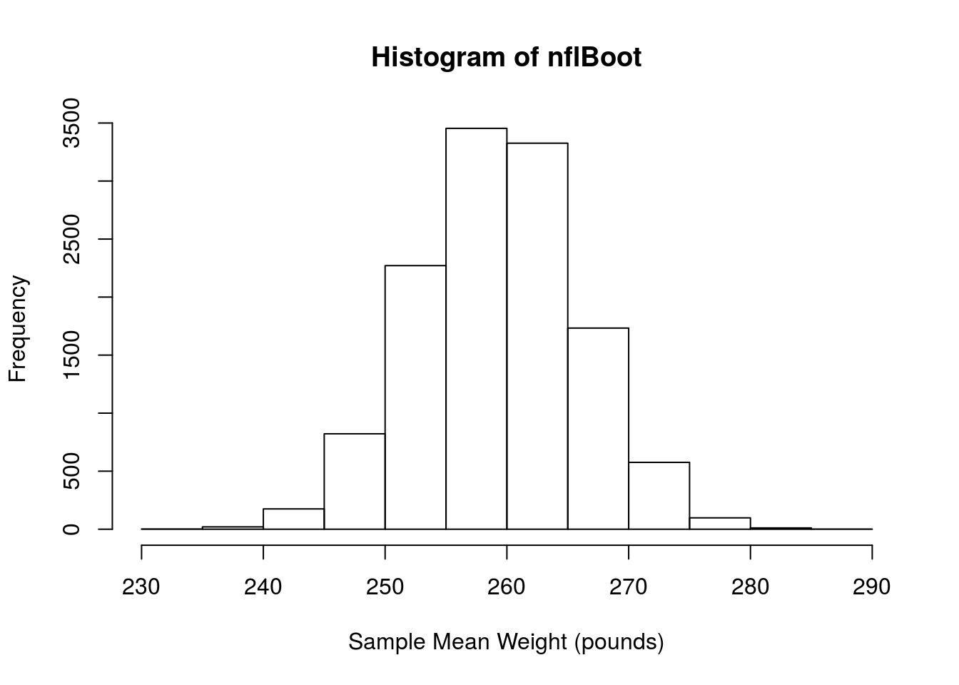
We can then estimate the standard error by finding the standard deviation
# Now calculate the standard error
sd(nflBoot)
## [1] 6.647575From this, we can calulate our 95% confidence interval:
# Caculate 95% CI
mean(nflSamples) + c(-2,2) * sd(nflBoot)
## [1] 245.9798 272.5702Importantly for this chapter, the standard error here should be (and is) very similar to the standard error calculated yesterday from the sampling distribution.
12.8.1 Try it out
Take a sample of 20 individuals from the AGE column from the mlb data, then use bootstrapping to estimate the standard error. Plot your results with a 95% confidence interval, and report the standard error you calculated.
Your output should look something like this:
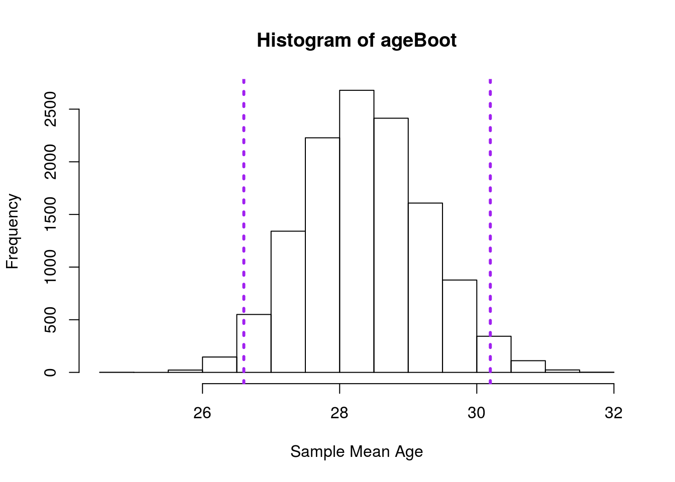
and you should get a standard error of around 0.899. However, bear in mind that slight differences in sampling will mean your results will not match these exactly.
12.9 Showing that this works
The below is not something I want you to copy or run, but is something that I want you to see. This is a loop of bootstrap loops. The complexity may start to show you what is possible, but more than that I want to demonstrate that this method works.
Below, I take thousands of separate samples, run bootstraps on each to calculate a 95% confidence interval, then show those that capture the true mean. We will see that it is very nearly 95%, just as it should be.
# Save the true mean
trueMean <- mean(mlb$Height)

isClose <- logical()

# Loop through the samples
for(i in 1:1178){
  tempSample <- sample(mlb$Height,
                       size = 40)
  tempMean <- mean(tempSample)

  # Bootstrap
  tempBootMean <- numeric()
  for(k in 1:1110){
    tempMLBboot <- sample(tempSample,
                          size = length(tempSample),
                          replace = TRUE)
    # Save the mean
    tempBootMean[k] <- mean(tempMLBboot)
  }
  seEst <- sd(tempBootMean)

  isClose[i] <- mean(tempSample) < trueMean + 2*seEst &
                mean(tempSample) > trueMean - 2*seEst
}

mean(isClose)
## [1] 0.9499151Note that almost exactly 95% (94.9915% to be exact) of the samples caputured the true mean within their confidence interval. This is important to note because going forward, we generally will be working from just a sample, and will not be able to verify which match and which do not.