29.1 Load today’s data

Start by loading today’s data. If you need to download the data, you can do so from these links, Save each to your data directory, and you should be set.

• montanaOutlook.csv
  • Data downloaded from The Data and Story Library
  • Originally from Bureau of Business and Economic Research, University of Montana, May 1992
  • Poll of Montana residence on their economic outlook
  • Contains some additional information about each respondent

# Set working directory
# Note: copy the path from your old script to match your directories
setwd("~/path/to/class/scripts")

# Load data
outlook <- read.csv("../data/montanaOutlook.csv")

29.2 Background

We have talked a lot about testing the the proportion of things with only two classes (e.g. heads or tails; and love or hate). However, it is often the case that we are interested in more than one category. For example, when we dealt with the conciousness state in the ICU data we could only test two categories at a time (e.g., “conscious” and not “conscious” or “conscious” vs “coma”). Today, we take the first step to analyzing multiple categories at once.

29.3 An example

For this, let’s look at the survey of Montana voters: in 1992, 209 people were surveyed about their current economic outlook (the outlook data). What if we want to know if each of the political parties are each getting their fair share of people in the poll? For now, let’s say that “fair” means that they are each equally represented in the poll.

# Look at number of people from each affiliation
nPol <- table(outlook$POL)
nPol

It looks like the Independents might be getting screwed. How can we test that? We could run a proportion test on each group, but that loses a lot of information. Instead, we can measure how far “off” each is all at once.

First, we need to set how many we expect for each. Here, we are expecting one-third to be from each of the three, so we set our expected number as one-third of the number of people that responded. Note that there are a few “NA” representing non-responses, we need to ignore these. So, what we want is the total number of people that responded, divided by the number of categories – which is just a mean.

# Calculate expected for each server
expected <- mean(nPol)
expected

## [1] 67.33333

So, we might have expected to get 67.33 people from each affiliation. Next, we want to figure out how far off we are:

# Calculate the difference
nPol -  expected

## 
##    Democrat Independent  Republican 
##    16.66667   -27.33333    10.66667

Then, since we have multiple groups, we want to add up all of the differences

# Sum them up
sum(nPol -  expected)

## [1] 1.421085e-14

Uh oh. They add up to almost exactly 0. To avoid this, we need to square each of the differences – otherwise the negative and positve offset.

# Square them
sum( (nPol -  expected)^2 )

## [1] 1138.667

That gives us a good measure of how far off we are, but it raises another problem. Consider what would happen if we just doubled our sample size. Our proportions would still be the same, but now this value would me much, much larger. We can see this by multiplying our counts (and expected value) by 2:

# What happens if we double our sample size?
sum( (2*nPol -  2*expected)^2 )

## [1] 4554.667

So, we need to scale for our sample size. This is usually accomplished by dividing each of the differences by the expected value. That way, each of the values becomes like a measure of the percentage we are off by.

# Scale by expected
sum( (nPol -  expected)^2 / expected)

## [1] 16.91089

We now have a good measure of how “wrong” our counts are. Now, obviously we wouldn’t have to look at each step once we know how the process works. We just calculated a “Chi-square” statistic, using this formula:

\[ \chi^2 = \sum{\frac{(Observed - Expected)^2}{Expected}} \]

This tells us to find the difference between the data we have observed and the values we expected (predicted) and sum them up. We square them to make sure that negative differences don’t negate positive differences, and we divide by to scale the effects. This gives us a measure of how different our data are from what we expect. We can then save that value to use ourselves:

# Save value
myChiSq <- sum( (nPol -  expected)^2 / expected)

But, once we get this value …. now what? Is 16.9 a big number? How can we figure it out? Well, one way is to simulate under the null and see what happens. Here, each time through the loop, we will sample the people from the political affiliations at equal rate. Then, we’ll calculate our Chi-Square statistic and see what the distribution looks like.

# Save names of political groups
polGroups <- names(nPol)

# Initialize
nullChiSq <- numeric()

# Run the loop
for(i in 1:12345){
  # Draw sample
  tempSample <- sample( polGroups, # sample from the groups
                        size = sum(nPol),
                        replace = TRUE)
  
  # Calc chi-sq
  # copied from above but remove intermediates
  tempTable <- table(tempSample)
  nullChiSq[i]  <- sum( (tempTable -  expected)^2 / expected)
  
}

# Visualize
hist(nullChiSq)
abline(v = myChiSq, col = "red3",lwd =3)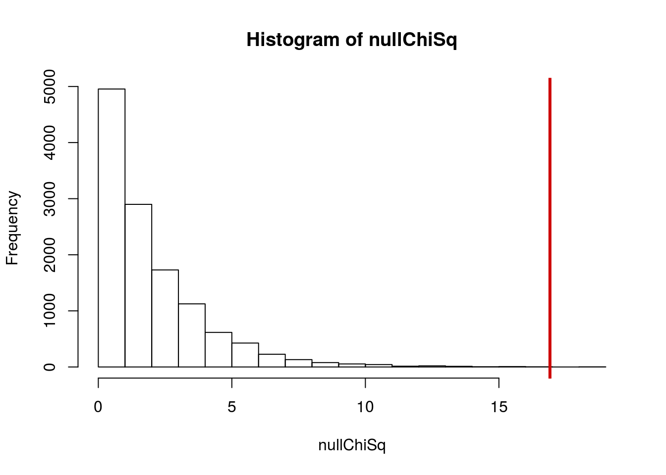

WOW. Very little of the distribution is past our value. It must be rare under the null (hint – that sounds like a p-value). So, let’s check that. How rare is it? What proportion of our nulls are as big or bigger?

# Calculate p
mean(nullChiSq >= myChiSq)

## [1] 0.0001620089

So, we can pretty confidently reject the null here. That is not likely to occur by chance. Note that we are only using a one-tailed test here. That is because, by squaring the differences, differences in any direction show up as positive numbers.

29.4 A small shortcut

Wouldn’t it be nice if we didn’t have to run that loop every time? Turns out, we don’t. Just like the normal- and the t-distributions, there is a distribution that estimates this pretty closely, unsurprisingly callled the Chi-Square distribution. In R, it is accessed with the functions pchisq(), qchisq(), and dchisq(). Like the t, these require a degrees of freedom argument.

Here, it is calculated a little differently. Instead of one less than the sample size, it is one less than the number of categories. That is because the data that actually goes in is just the counts per category. An easy way to think about this (and why it is called degrees of freedom) is that, with three categories, we can “freely” set the values of two of them, but then the third has to be what ever is left. So, we have one less “free” category than we have categories.

To see this in our case, let’s lay a curve on top of our histogram using curve() like we did for the normal.

# Show the chisq distribution
hist(nullChiSq, freq = FALSE, breaks = 40)
curve(dchisq(x, df = 2),
      add = TRUE, xpd = TRUE,
      col = "green3", lwd = 4)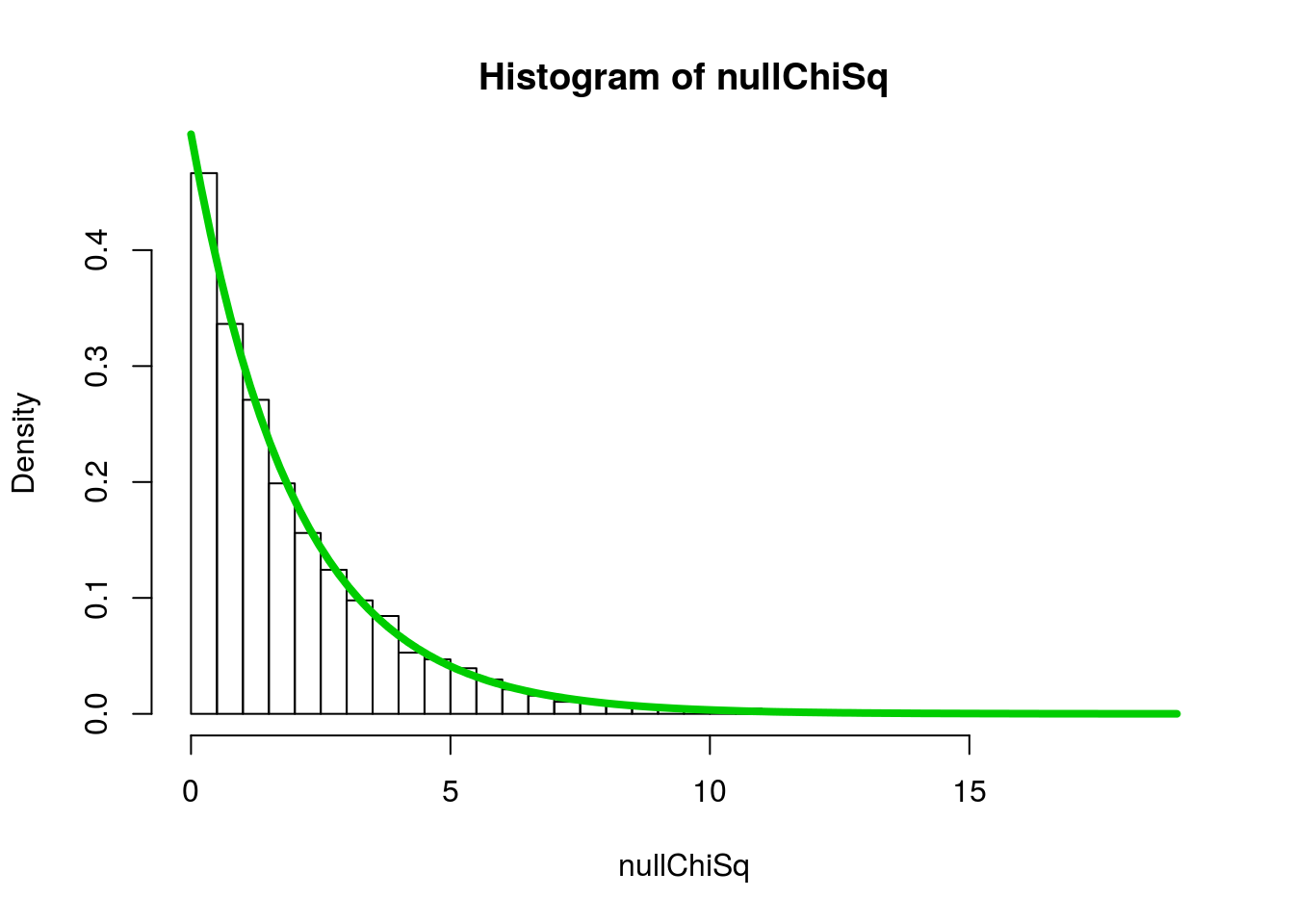

Like with the t, as the degrees of freedom go up, the shape gets more like the normal. Let’s see:

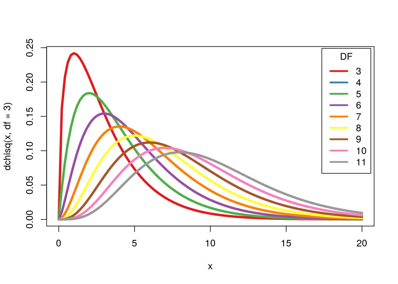
This also shows us one interesting difference with this distribution: we don’t actually “expect” values that are too similar to the expected values when we get more categories. For example, with 11 categories, it would be rather surprising to get a chi-squared value of close to 0[*] Mendel, the founder of genetics, has been accused of falsifying or manipulating data because his data were too close to the expected counts. However, careful re-anlaysis suggests that a few moderate un-stated assumptions account for the data being ‘too good.’ For more detail see http://en.wikipedia.org/wiki/Gregor_Mendel#Controversy and follow the relevant citations. .

# Calculate P
1 - pchisq(myChiSq, df = 2)

## [1] 0.0002127388

# Compare to sampling
mean(nullChiSq >= myChiSq)

## [1] 0.0001620089

29.5 Assumptions

The one assumption of the Chi-Squared approximation we need to be most aware of is that it does not work well for low expected counts. As a general rule, we need to expect at least 5 counts in each category for the Chi-Square approximation to be valid.

29.6 Shorter cut

As you have probably guessed, there is an even shorter cut available: chisq.test(). Just like prop.test() and t.test(), this allows us to pass in some data, and get our relevant statistics out. Look at the help (and the examples we cover for the next section) for more details, but for now, this will work:

# Run the test
chisq.test( nPol )

## 
##  Chi-squared test for given probabilities
## 
## data:  nPol
## X-squared = 16.9109, df = 2, p-value = 0.0002127

This gives us the basics, but we can get more details still, which we will explore next tutorial. Note, in particular, that the p-value is identical to what we calculated using pchisq() and that it automatically calcluated our degrees of freedom and chi-squared statistic.

29.7 With a different null

Finally, we don’t always think that all categories are equally likely. Sometimes, everything being equal would be very unusual. In this case, what if there really are fewer independents in the population? Now, we’d no longer expect to have the same number of independents as Democrats and Republicans. To show this, imagine that we know that, in Montana, 40% of people are Democrats, 20% are Independents, and 40% are Republicans. We can then change our “expected” values to match this proportion. We would then expect to get those proportions from our sample as well.

# Save the population proportions
expProp <- c(0.4, 0.2, 0.4)

expected <- expProp * sum(nPol)
expected

## [1] 80.8 40.4 80.8

We can then look at how close our observed data are to this new expectation:

# How far off is each
nPol -  expected

## 
##    Democrat Independent  Republican 
##         3.2        -0.4        -2.8

That is a whole lot closer. Here, we see that we have 3.2 more Democrats than expected, which is a lot closer than before. So, we can calculate a new chi-square value.

# store the result
myChiSq <- sum( (nPol -  expected)^2 / expected)
myChiSq

## [1] 0.2277228

Now our statistic is quite small. What is our p-value here?

# Calculate p
1 - pchisq( myChiSq, df = 2)

## [1] 0.8923816

So, now we wouldn’t reject the null. If the population really is set up like this, it could explain the pattern. Recall, however, that this does not mean that the population definitely is exactly those proportions of each party. We simply do not reject the null – we can never accept it.

We can get there even faster using our shorter cut. By passing the argument p = to chisq.test() we can set any null distribution we want. You must set one probability for each of the categories (in order) and the value must sum to 1 (because these categories make up all of the possible outcomes). If you don’t pass in a value for p =, R assumes that your null is equal proportions, which is why we didn’t need to set it for our first example.

# run test
chisq.test(nPol, p = expProp )

## 
##  Chi-squared test for given probabilities
## 
## data:  nPol
## X-squared = 0.2277, df = 2, p-value = 0.8924