An introduction to statistics in R
A series of tutorials by Mark Peterson for working in R
Chapter Navigation
- Basics of Data in R
- Plotting and evaluating one categorical variable
- Plotting and evaluating two categorical variables
- Analyzing shape and center of one quantitative variable
- Analyzing the spread of one quantitative variable
- Relationships between quantitative and categorical data
- Relationships between two quantitative variables
- Final Thoughts on linear regression
- A bit off topic - functions, grep, and colors
- Sampling and Loops
- Confidence Intervals
- Bootstrapping
- More on Bootstrapping
- Hypothesis testing and p-values
- Differences in proportions and statistical thresholds
- Hypothesis testing for means
- Final thoughts on hypothesis testing
- Approximating with a distribution model
- Using the normal model in practice
- Approximating for a single proportion
- Null distribution for a single proportion and limitations
- Approximating for a single mean
- CI and hypothesis tests for a single mean
- Approximating a difference in proportions
- Hypothesis test for a difference in proportions
- Difference in means
- Difference in means - Hypothesis testing and paired differences
- Shortcuts
- Testing categorical variables with Chi-sqare
- Testing proportions in groups
- Comparing the means of many groups
- Linear Regression
- Multiple Regression
- Basic Probability
- Random variables
- Conditional Probability
- Bayesian Analysis
Differences in proportions and statistical thresholds
15.1 Load today’s data
Start by loading today’s data. If you need to download the data, you can do so from these links, Save each to your data directory, and you should be set.
- icuAdmissions.csv
- Data on patients admitted to the ICU. Note this file has been updated, so you should download it again.
# Set working directory
# Note: copy the path from your old script to match your directories
setwd("~/path/to/class/scripts")

# Load data
icu <- read.csv("../data/icuAdmissions.csv")
15.2 Overview
Often times it doesn’t make sense to test a null hypothesis for a proportion. For example, what null hypothesis would you set for the proportion of people that die after admission to the ICU? You might have a national standard to compare against, in which case you could test whether or not a particular hospital differed from the national value. However, even that might not be very informative, especially if the hospital in question is an odd one for some reason (e.g., average patient age is different, more trauma, etc.).
However, in those cases, we might be interested in comparing the proportion between two different cases. For example, we might want to know if a particular treatment was related to higher (or lower) survival. In this chapter, we explore this type of analysis.
Further, we will discuss more about the rules for interpretting p-values.
15.3 Survival by Type of Admission
Let’s get specific here. We want to know whether patients are more likely to die following admission for “emergency” or “elective” procedures. These data are given in the Type column of the icu data and the Status column tells whether patients “lived” or “died”. We need to first specify our null and alternative hypotheses.
What is the simplest, most boring, status quo thing that could be true about the relationship between these values? … That there is no difference between them. This will be our null hypothesis.
For our alternate we then have to decide whether to use one tail or two. Personally, I think that a two-tailed test is almost always appropriate. In this case, you could argue that we expect the difference to go in one direction, but I contend that I could make a just-so story in either direction. “Elective” are less likely because it suggests that there is not an emergent case, or “Elective” are more likely to die because only people in distress would choose to go into the ICU. If you choose to use a one-tailed test make sure that you can (and do) defend that choice clearly. If there is ever doubt, a two-tail test is likely appropriate.
Together this gives us these hypotheses.
H0: proportion of “elective” patients that die is equal to the proportion of “emergency” patients that die.
Ha: proportion of “elective” patients that die is not equal to the proportion of “emergency” patients that die.
Note here that we did not set the thing we are interested in (and even suspect may be true) as the null. The null is the “status quo” and the thing we “try” to reject. It also must be a point estimate, that is a single value. Here, we use no difference, which is equivalent to “0”. No where in the question do we have any similar predicted value for the difference between the two Types of admissions that might serve as a similar point estimate.
15.3.1 Describing data
As always, we need to look at our data. Because we are investigating two categorical variables (and are interested in proportions), start by making a simple table.
statType <- table(icu$Status, icu$Type)
addmargins(statType)| elective | emergency | Sum | |
|---|---|---|---|
| died | 2 | 38 | 40 |
| lived | 51 | 109 | 160 |
| Sum | 53 | 147 | 200 |
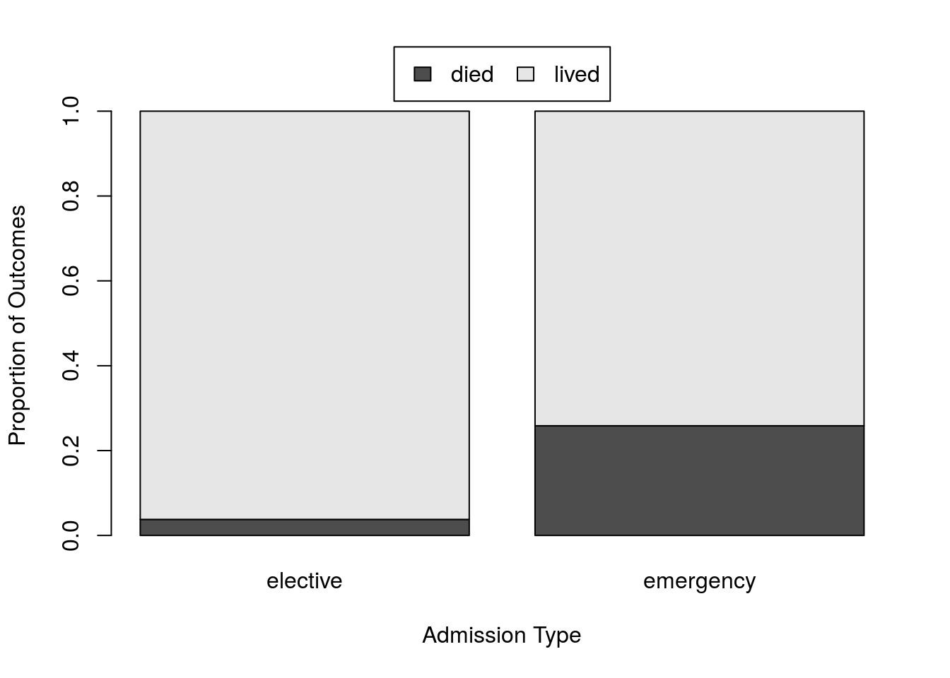
That sure looks like a big difference. However, the difference in numbers for each Type mask some of the difference. So, we should calculate the proportions that died in each. There are (as always) a lot of ways to do this. For our purposes, using prop.table() might make the most sense.
# Show relative survival
statTypeRates <- prop.table(statType, 2)
# Plot it
barplot(statTypeRates)| elective | emergency | |
|---|---|---|
| died | 0.0377358 | 0.2585034 |
| lived | 0.9622642 | 0.7414966 |
Because the table output has named rows and columns, we can access a specific cell by giving the row and column names. We can then save the difference between the two like this:
# Store the difference to use for testing
diffProp <- statTypeRates["died", "elective"] -
             statTypeRates["died", "emergency"]
# View the difference
diffProp
## [1] -0.2207676Note that, were we less morbid, we could calculate survival rates instead of morbidity rates by trading "died" for "lived" in the line above. Either is appropriate, we just need to make sure that we do the same when we construct our null distribution.
Of note, there are other ways that we could save the difference in the proportion. This is just the one that I find most intuitive and least susceptible to error. It is also the one that I think is likely to be easiest to manage when we transition to other data types soon. However, if there is a method that you prefer, feel free to use that instead.
15.3.2 Create a null distribution
Now, if we want to ask if this difference in proportions is “statistically significant,” we need to create a null distribution. For the simple case of one proportion, that was easy. We just specified the propotion from our null hypothesis. Here, our null hypothesis is that the difference in the proportions will be 0.
Said another way, our H0 states that the likelihood of dying is not related at all to the type of admission. This makes our null distribution easy to make. Instead of specifying a probability, we can simply sample from the Status column without regard to the Type column and see how different the two proportions are in many samples.
It is impotant to note here that we are sampling from Status and not from Type because our hypothesis is about what happens in Status given Type, not the other way around. This seems like a minor point, but is important to remember because, as before, we need to keep our sample sizes consistent, and that includes the number in each group[*] There is a related debate about whether sampling should be with or without replacement from Status. The arguments are many and are largely philosophical rather than mathematical. For any comparision involving two variables (e.g., comparing groups), it is arguably as approriate (or even more appropriate) to sample without replacement to keep the exact values the same and only change the relationship between the two variables. Here, I tend to stick with sampling with replacement largely because it makes it easier to rememeber to sample with replacement in cases where that is necessary. . So, we don’t want the number of “elective” and “emergency” admissions changing.
As before, we start with making a simple sample before building our loop. Start by thinking about how you might do this by hand; the steps are simple. First, sample the statuses (note that we this has nothing to do with Type). Second, build a table to compare the sampled Statuses with the Types. Finally, calculate the difference between the proportions.
# Sample the status
tempStatus <- sample(icu$Status,
                     size = nrow(icu),
                     replace = TRUE)
# Construct a table
#    I copied this from above,
#    changing only what statuses we use
tempTable <- table(tempStatus, icu$Type)
tempRates <- prop.table(tempTable, 2)

# Calculate the difference
tempRates["died", "elective"] -
   tempRates["died", "emergency"]
## [1] -0.03953279Now, we can simply create a loop, copy that sample into it, and make sure that we save the sample statistic (the difference in proportions).
# intialize variable
statTypeNull <- numeric()

for(i in 1:12345){
  # Sample the status
  tempStatus <- sample(icu$Status,
                     size = nrow(icu),
                     replace = TRUE)
  # Construct a table
  #    I copied this from above,
  #    changing only what statuses we use
  tempTable <- table(tempStatus, icu$Type)
  tempRates <- prop.table(tempTable, 2)

  # Calculate the difference
  # Again, copied, only changing variable names
  statTypeNull[i] <- tempRates["died", "elective"] -
                       tempRates["died", "emergency"]
}
Now, we have a full null distribution for the difference in proportions. As always, we want to look at it and make sure that it makes sense.
# Plot the null
hist(statTypeNull,
     main = "Null distribution for difference in survival",
     xlab = "Difference in proportion")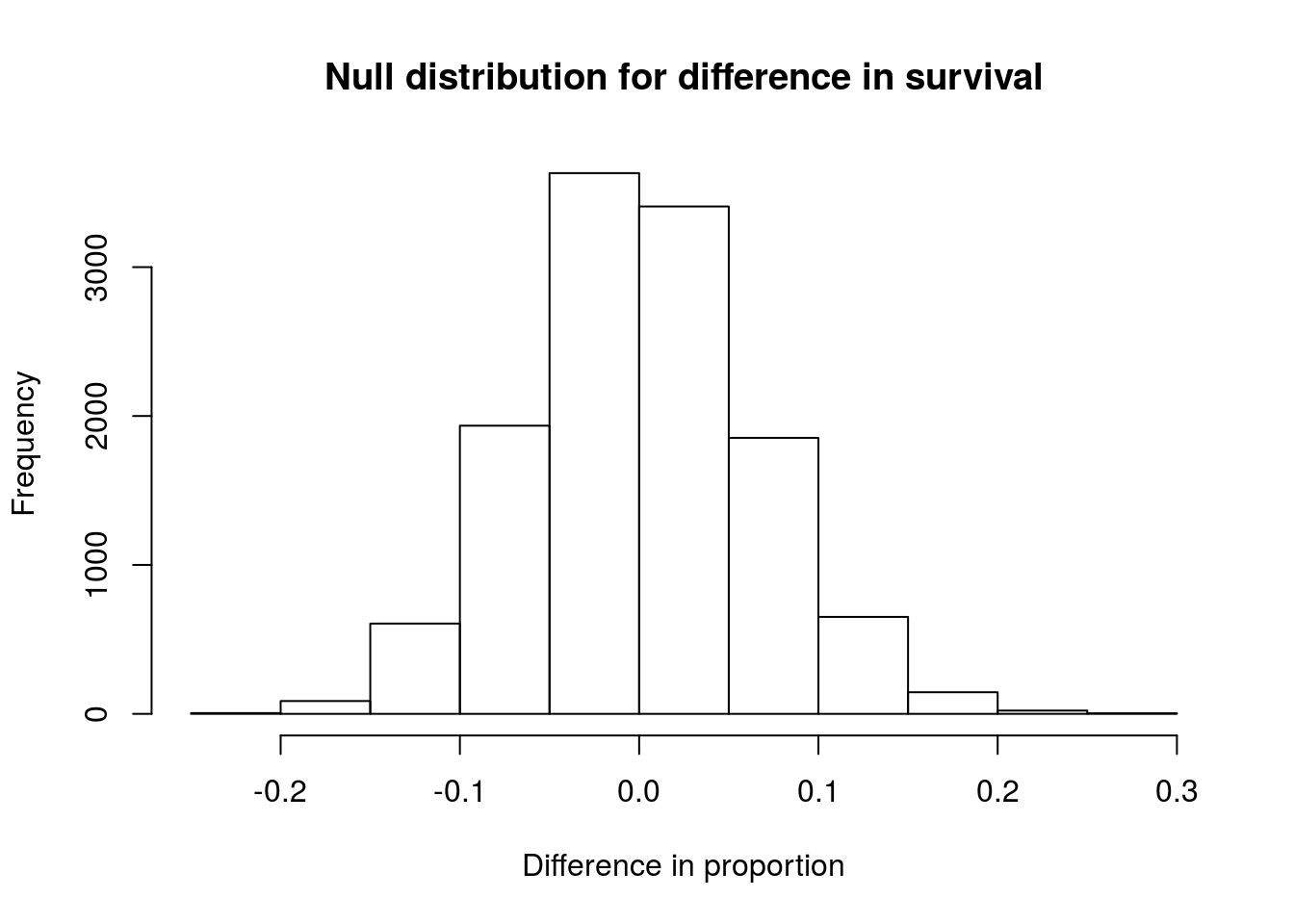
As expected, the distribution is centered around 0, or no difference. The distribution looks symmetric, and does not suggest any problems.
15.3.3 Calculate a p-value
Now, we can add lines representing our actual recorded difference (saved above). Note that, because we have a two tailed distribition, we include both the actual difference and the difference in the opposite direction.
abline(v = c(diffProp,
             -diffProp))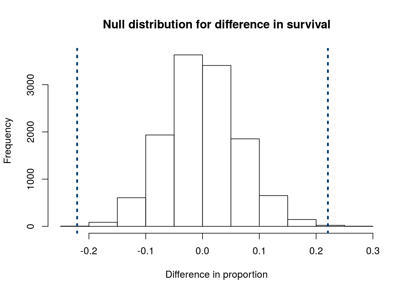
It seems clear that very few of the null distributions are outside of those lines. However, we want to put an exact number on it. So, we need to calculate how many values are as extreme as, or more extreme than, our observed data. If our Ha were one tailed, we would only need to calculate the number more extreme in that direction. However, when we use a two-tailed Ha, we need to test those more extreme in either direction. For that, we could either count them up separately and add them together, or we can use the | character (the “pipe”, usually above the “Enter” key) which means “or” when testing logicals. As always, the mean() is counting how many match, then dividing by the number of samples in our null distribution.
# Test proportion more extreme in either diretion
pMoreExtreme <- mean(
  statTypeNull <=  diffProp |
  statTypeNull >= -diffProp
  )

pMoreExtreme
## [1] 0.001053058This is an incredibly small value, and I think that we can all agree that we can reject our H0 of no difference between the proportion of patients that die among “elective” and “emergency” admissions.
15.4 Put it together
To see these pieces in action together, let’s try looking at the difference in survival by sex. Specifically, are men more likely than women to die after admission to the ICU? First, we need to explicitly state our hypotheses
H0: proportion of men that die is equal to the proportion of women that die.
Ha: proportion of men that die is not equal to the proportion of women that die.
As before, the null is our “status quo” of no difference. If we reject it, then we might believe there is a difference.
Next, we need to look at our data. Note that this, like most of the lines in this section, is copied from above, only changing variable names.
statSex <- table(icu$Status, icu$Sex)
addmargins(statSex)| female | male | Sum | |
|---|---|---|---|
| died | 16 | 24 | 40 |
| lived | 60 | 100 | 160 |
| Sum | 76 | 124 | 200 |
That looks like it might be a little different, but the different values again make it hard to say. So, let’s calculate the proportions and plot them.
# Show relative survival
statSexRates <-prop.table(statSex, 2)
# Plot it
barplot(prop.table(statSex, 2))| female | male | |
|---|---|---|
| died | 0.2105263 | 0.1935484 |
| lived | 0.7894737 | 0.8064516 |
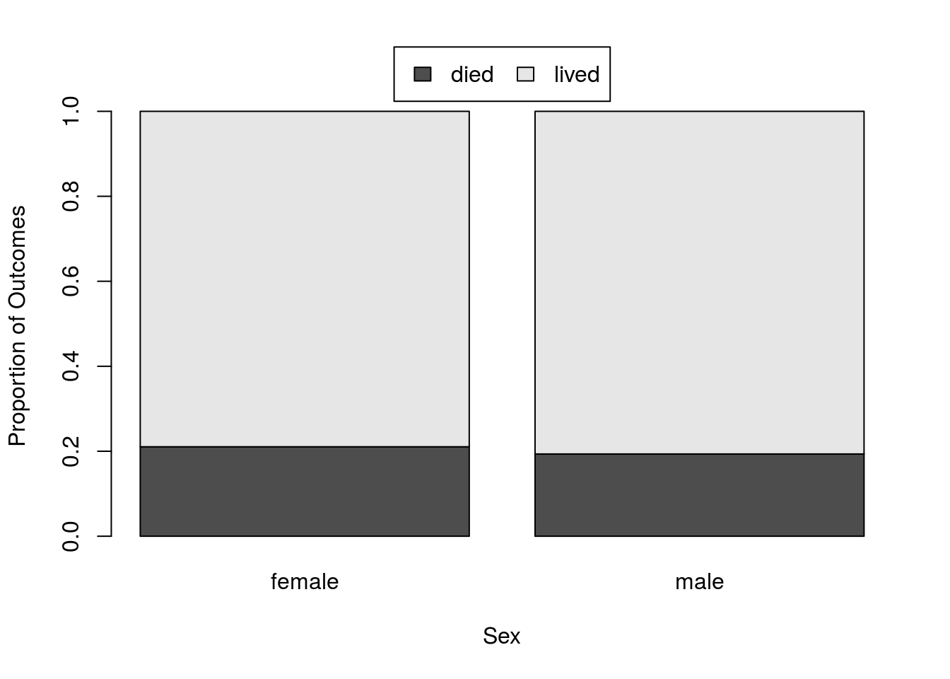
Yikes, not much difference there, but let’s still keep moving forward. We need to save the difference in proportion next. Again, this is copied from above with “male” and “female” now replacing the types of admissions
# Store the difference to use for testing
diffProp <- statSexRates["died", "male"] -
             statSexRates["died", "female"]
# View the difference
diffProp
## [1] -0.01697793Now, to ask if this difference in proportions is “statistically significant,” we need to create a null distribution. Because we have a loop from above, we can simply copy that loop and make changes to it.
# intialize variable
statSexNull <- numeric()

for(i in 1:13546){
  # Sample the status
  tempStatus <- sample(icu$Status,
                       size = nrow(icu),
                       replace = TRUE)
  # Construct a table
  tempTable <- table(tempStatus, icu$Sex)
  tempRates <- prop.table(tempTable, 2)

  # Calculate the difference
  statSexNull[i] <- tempRates["died", "male"] -
                       tempRates["died", "female"]
}
Now, we want to look at the distribution and make sure that it makes sense.
# Plot the null
hist(statSexNull,
     main = "Null distribution for difference in survival",
     xlab = "Difference in proportion")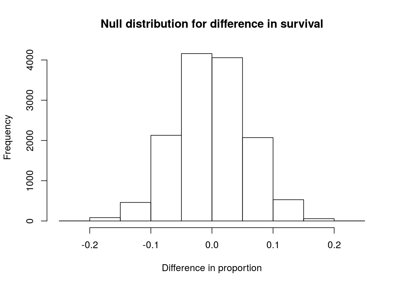
As expected, the distribution is centered around 0, or no difference. The distribution looks symmetric, and does not suggest any problems.
We can then add lines representing our actual recorded difference.
abline(v = c(diffProp,
             -diffProp))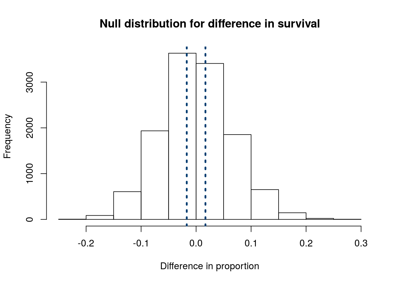
It seems clear that almost all of the values from the null distribution are more extreme than our observed values. To put an exact number on that:
# Test proportion more extreme in either diretion
pMoreExtreme <- mean(
  statSexNull <=  diffProp |
  statSexNull >= -diffProp
  )

pMoreExtreme
## [1] 0.7784586This is a rather large value – about 80% of samples from our null distribution gave differences as large as, or larger than, our observed difference. I think that we can all agree that we can not reject our H0 of no difference between the proportion of patients that die between men and women.
Importantly, this does NOT mean that the there is definitely no difference in the mortality rates between the sexes. All it means is that we do not have enough evidence to say that there is a difference. If the true difference were very small, we would also expect to get very similar data.
15.5 Try it out
Try this out on your own. Is there a difference in the mortality rate (proportion that die) between patients that get “surgery” and those that get “medical” service? The column Service lists the type or treatment the patient go.
Follow the steps from above, including stating your null and alternative hypotheses. You should get a null distribution that looks something like this:
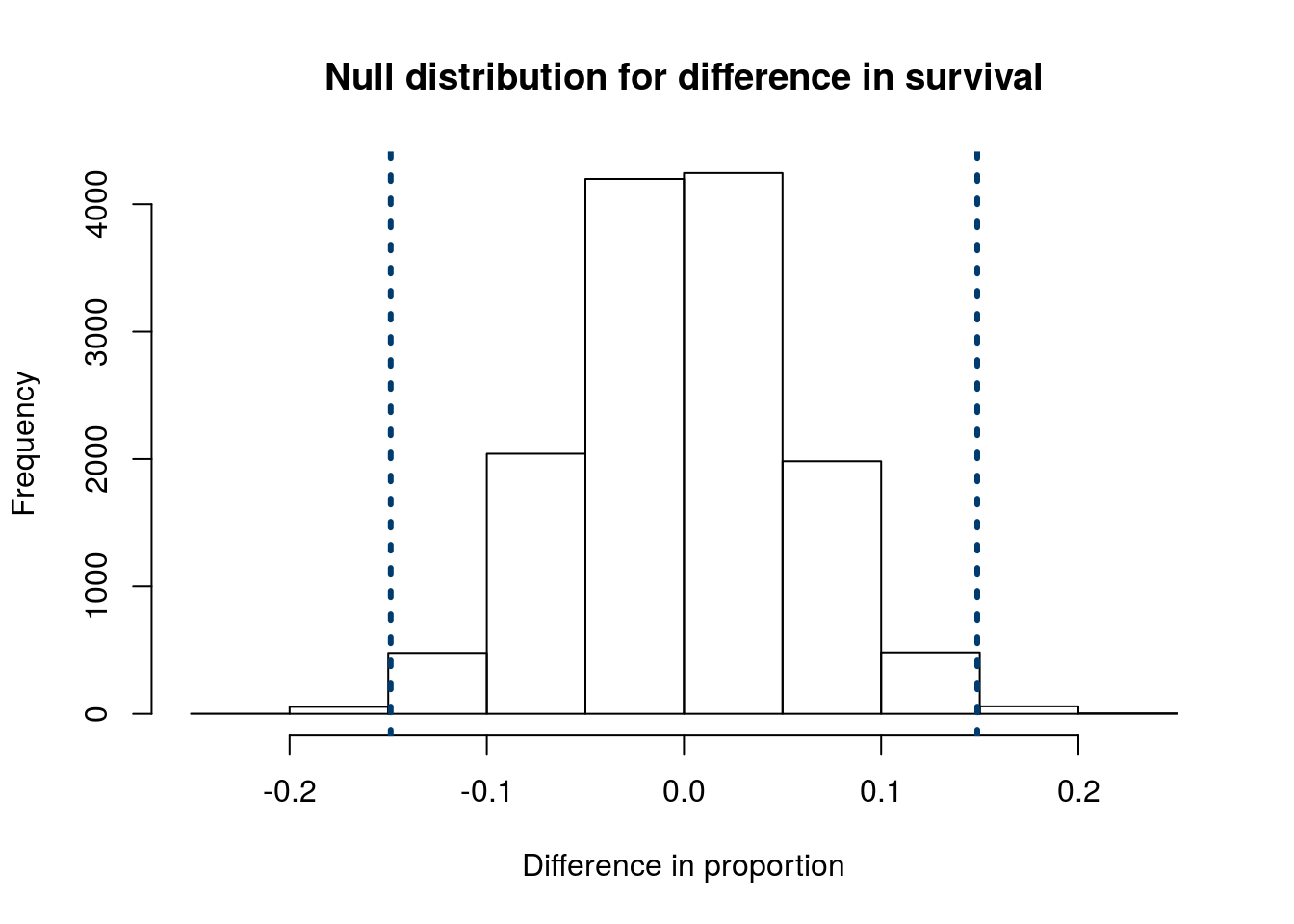
and a p-value of about 0.01. What can you conclude about the null hypothesis? Can you reject it?
15.6 How small is small “enough”
Above, there have been three examples:
- We can clearly say we suspect a difference in mortality between “elective” and “emergency” admisssions
- We clear can not say there is a difference in mortality between men and women (though we also can not say that there is no difference)
- The case for the type of Service may be a little murkier. Is 1 in 100 rare “enough” to reject the null?
Where is the line between the two extreme examples?
The first two examples are illustrative of the extremes, but they don’t do much to help us understand what is going on in between them. For that, we need to take a small step back and think about our goals and where they can go wrong.
Our goal is to accurately determine whether or not H0 explains our data. This can go right in two ways (we correctly reject or correctly do not reject). However, it can also go wrong in two ways (we incorrectly reject or incorrectly do not reject). In a table, that looks like this
| Reject H0 | Do not reject H0 | |
|---|---|---|
| H0 is True | Type I error | No error |
| H0 is False | No Error | Type II error |
The level we set at which to reject (commonly called α or alpha), is a balance between these two error types. If we set it too strictly (very small) we will be likely to make Type II errors (incorrectly not rejecting). If we set it to leniently (very large) we will be likely to make Type I errors (incorrectly rejecting). No α level is safe from these errors, but we can balance their risks.
For things where Type II error is very dangerous (e.g. medical tests for serious diseases) we may set laxer thresholds. For things where Type I error is a very big deal (e.g. claiming to have identified a new physics particle), we might set more stringent thresholds.
In reality, the balance you strike will be, at least in part, determined by the field you are working in. For most tests you will run, you will be using α levels of 1%, 5%, or 10%. Of these thresholds, 5% is the most common (though, that doesn’t make it right).