35.1 Load today’s data

No data to load for today’s tutorial. Instead, we will be using R’s built in randomization functions to generate data as we go.

35.2 Background

Until now, we have just been looking at the outcome of a trial – is it heads, red, a one, etc. However, in many situations, we are likely to be interested in some numerical measure of the outcome. In our dice example, we might want to track the value of the faces of the die (e.g. for a game).

In such situations, we may be interested in predicting the value of the variable, such as the face of a die, the number on a card, or the amount of money that we will get paid. The rules of probability that we have already explored still hold, but in this section we will focus just on handling the numeric values after being given the probability of each outcome (rather than solving for those probabilities as well).

Random variables can either be discrete or continuous. In the examples in this chapter, we will focus on discrete random variables. That is, there are a specific number of possible outcomes, each of which has some defined probability of occurring. This is most similar to the probability rules we have been learning until now.

However, random variables that we encounter in everyday life are often continuous – meaning that they can take on any value, usually within a range. This might be something like the number of seconds it takes a fast food restaraunt to serve your food, or the amount of money thrown into a water fountain at the mall. The variables are usually modelled with with the normal model, as it fits most variables well enough. All of the rules about combining random variables described below for discrete variables apply directly to continuous variables as well, but their application is beyond the scope of this class.

35.3 Entering data

For this section, we will use a simple example involving bonus points for a class. Each player has the chance to get 5, 1, or 0 bonus points, the probabilities of each value are:

	Payout	Probability
big	5	0.15
small	1	0.25
nothing	0	0.60

For all of the things we need, we need to set our potential values of X, the probabilities of each value, and then combine them in some way. So, here, let’s set the values directly, then see a couple shortcuts.

# Set payouts
payouts <- c(5, 1, 0)

# Set probabilities
probs <- c(3/20, 5/20, 12/20)

# Display them
data.frame(payouts, probs)

##   payouts probs
## 1       5  0.15
## 2       1  0.25
## 3       0  0.60

As an aside, that was a slightly obnoxious way to have to enter the probabilities. Instead, we could divide each by 20 at the end like this:

# Divide each by 20 at the end
c(3, 5, 12) / 20

## [1] 0.15 0.25 0.60

Or, we could use relative probabilities, then divide by the sum. This way, we ensure that our probabilities always add to 1 (they have to, by definition). Here, it is functionally the same:

# Store temp relative probabilities
tempP <- c(3, 5, 12)

# See the sum
sum(tempP)

## [1] 20

# Divide each by that sum (same as above)
tempP / sum(tempP)

## [1] 0.15 0.25 0.60

However, this is often helpful if we are doing something quick where we know the relative relationships, but haven’t bothered to figure out the actual probabilities. For example, what if I told you that you were twice as likely to get 1 point as 5, and 5 times as likely to get 0 points as 5? We could enter that as below:

# Store temp relative probabilities
tempP <- c(1, 2, 5)

# See the sum
sum(tempP)

## [1] 8

# Divide each by that sum (same as above)
tempP / sum(tempP)

## [1] 0.125 0.250 0.625

all without having to do the calculations by hand.

35.4 Expected Value

The expected value of a random variable (a fancy term for the mean outcome) is calculated as:

\[ E(X) = \sum x * p(x) \]

Where E(X) is the expected value, x is each potential value of X and p(x) is the probability of each x. In words, the mean value of X is each potential value of X times its probability of occurring.

In R, we can do this fairly straightforwardly. Just multiply our payouts by our probs and take the sum – just like in the equation. Recall that, when working with vectors that are the same length, R does the arithmetic by matching up the vectors (that is, it multiplies the two first values, then the two second values, and so on).

# Calculate expected value
expVal <- sum( payouts * probs)

# Display
expVal

## [1] 1

We get an expected value of 1, and we can even see the intermediate step as if we had done this by hand:

payouts * probs

## [1] 0.75 0.25 0.00

This is how much each contributes to the expected value (the mean). You can see that, no matter how likely it is that we get 0, it always contributes 0 to the expected value.

35.5 Spread

We calculate the spread of a random variable in much the same way as we calculate the spread of any variable. The difference is that we don’t have all of the values. Instead we have probabilities for each potential value. Thus, the variance of a random variable is defined as:

\[ var(X) = \sum (x - E(X))^2 * p(x) \]

and the standard deviation is, as always, the square root of the variance. So, we can again just plug our information into the equation:

# Calculate variance
varX <- sum( (payouts - expVal)^2 * probs  )

Here, we get 3. We can get the standard deviation by taking the square root.

# Get the standard deviation
sqrt( varX )

## [1] 1.732051

35.6 Adding to the payouts

Adding to the payouts is easy – we just add our constant to the payouts and recalculate. Here, I will save the new payouts as a new variable, but we could also just do this in each of the equations

# Add 2 to each payout
newPayouts <- payouts + 2
newPayouts

## [1] 7 3 2

Now, just plug newPayouts in everywhere:

# Calculate expected value
newExpVal <- sum( newPayouts * probs)
newExpVal

## [1] 3

# Calculate variance
newVarX <- sum( (newPayouts - newExpVal)^2 * probs  )
newVarX

## [1] 3

# Get the standard deviation
sqrt( newVarX )

## [1] 1.732051

So, we can see that our expected value went up by the constant and that the variance and standard deviation did not change. This holds for any such change addition, or subtraction, of a constant (A below) to a random variable.

E(X ± A) = E(X) ± A

Var(X ± A) = Var(X)

sd(X ± A) = sd(X)

35.7 Multiply by a constant

Oftentimes we may want to multiply by a constant instead. For example, in 2001, the payouts on Jeopardy! doubled. In this case, we can see the effect just as easily as we did for adding a constant. We simply multiply by our constant and recalculate. Here, I will save the new payouts as a new variable, but we could also just do this in each of the equations.

# Multiply each payout by 2
newPayouts <- payouts * 2
newPayouts

## [1] 10  2  0

Now, just plug newPayouts in everywhere:

# Calculate expected value
newExpVal <- sum( newPayouts * probs)
newExpVal

## [1] 2

# Calculate variance
newVarX <- sum( (newPayouts - newExpVal)^2 * probs  )
newVarX

## [1] 12

# Get the standard deviation
sqrt( newVarX )

## [1] 3.464102

So, we can see that our expected value went up by a factor of the constant (it doubled), which should match our intuition. However, the variance went up by the square of the constant (meaning that the standard deviation went up by the constant). Looking at our equation for the variance, we can see that this is because when we double the values, we double the difference between each and the new expected value. That difference is then squared, leaving the variance increased by a factor of the constant squared (here 2² = 4; the same would hold if we tripled the values: 3² = 9). Because the standard deviation is the square root of the variance, we can see that it goes up by a factor of the constant

E(X * A) = E(X) * A

Var(X * A) = Var(X) * A²

sd(X * A) = sqrt( Var(X) * A²) = sd(X) * A

35.8 Combining two variables

Another common occurance that we encounter is seing what happens when we sample a random variable many times. For example, what is the sum of the dice if we roll them twice? Or, in our example, what are the total number of points one if you play the game twice? You will likely notice here that this sounds a lot like our sampling distribution of means. The only difference is that we would need to divide by the number of samples to get a mean instead of a sum. This is not a coincidence, and you will notice that the equations here are very similar to the shortcuts we learned to estimate the standard errors in other chapters. This is not a coincidence. The math behind (and beyond) this chapter is what led to the shortcuts we learned.

We could figure out how to combine all of the various possible outcomes (using the multiplication rules for probability), but that becomes infeasible with even a moderate number of possible outcomes. Instead, we will just use some formulas that have already been developed. Specifically, that the expected value and variance of the sum of two variables is the sum of their separate expected values and variances.

var(X ± Y) = var(X) + var(Y)

Note here that we always add the variances, whether we are adding or subtracting Y from X. So, for the example where each student plays twice, we see that our expected value is just doubled (the sum of the two expected values), just like when we doubled each prize. The variance, however, is different than when we doubled each:

# Calculate combined expected value
expVal + expVal

## [1] 2

# Calculate combined variance
varX + varX

## [1] 6

# Calculate combined standard deviation
sqrt( varX + varX )

## [1] 2.44949

Note that the combined variance went up by a lot less than when we doubled the payouts. This is why insurance companies and casinos make money: when there are lots of independent trials (cars, slot pulls, etc.), the expected value adds the same as if you just multiplied by the number of trials, but the variance (and sd) go up much more slowly, leveling off the risk.

We can see why this is the case by simulating many sets of trials. Here, I use one loop to store the outcomes of both a double value (what we did when multiplying) and two indpendent values. We will sample from each set of payouts, with the probability set to probs to match our example.

# intialize variables
doubledOut <- twoTrialOut <- numeric()

for(i in 1:12345){
  # Sample for the doubled values
  doubledOut[i] <- sample(newPayouts,
                          size = 1,
                          prob = probs)
  
  # Sample for the two independent -- note need sum
  twoTrialOut[i] <- sum( sample(payouts,
                                size = 2,
                                replace = TRUE,
                                prob = probs))
}

Now, let’s use table() to look at the outcomes:

# View the outcomes of doubled
table(doubledOut)

## doubledOut
##    0    2   10 
## 7419 3120 1806

# View the outcomes of two trials
table(twoTrialOut)

## twoTrialOut
##    0    1    2    5    6   10 
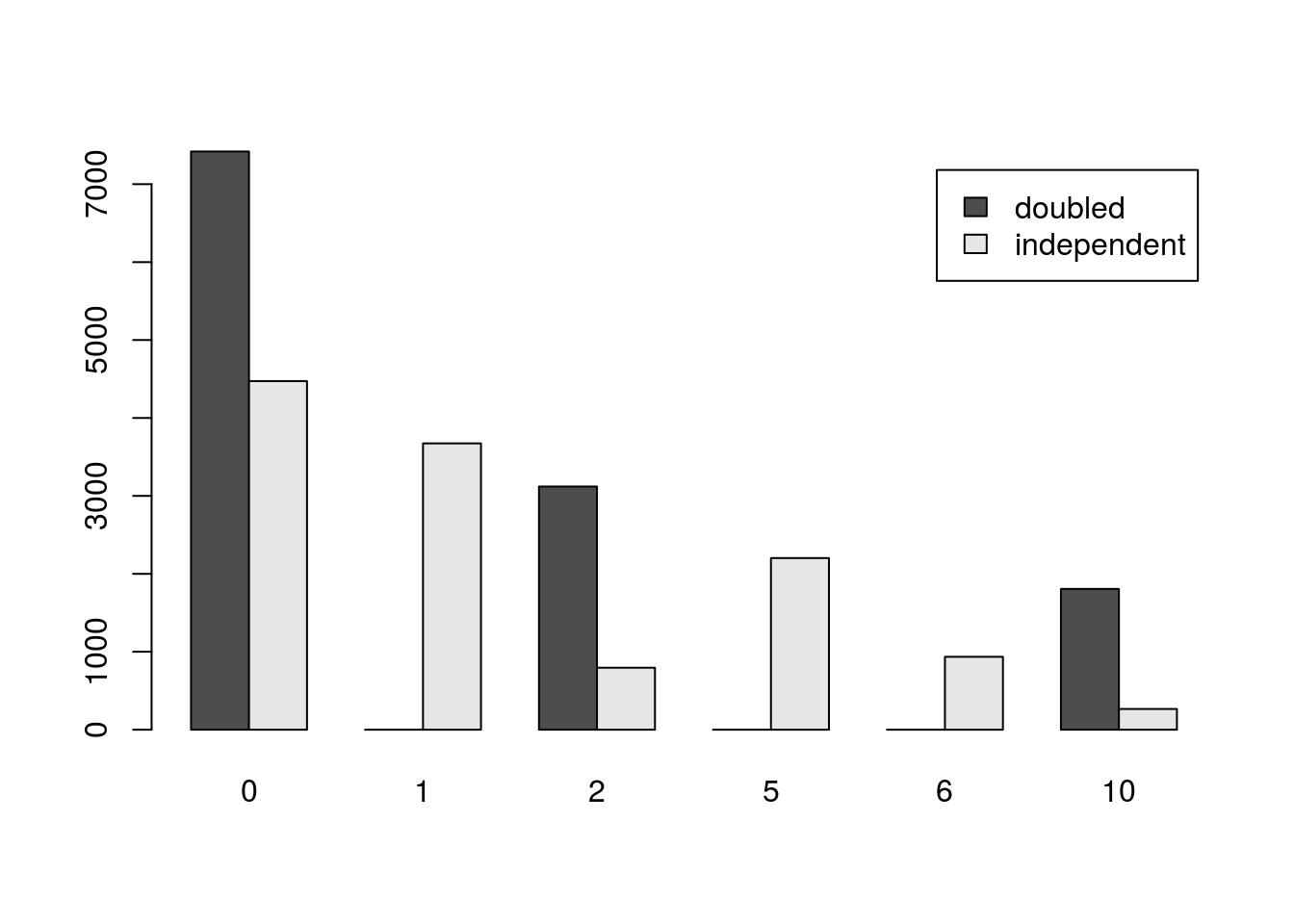
## 4473 3674  795 2202  935  266

Note how many more possible values occur when the trials are independent, and how many fewer 10’s there are. We can calculate the means and sds of these outcomes to show that the equations above work. (This is something I often do when I am not sure if I am using an equation right. It is a good way to check.)

# Mean of doubled
mean(doubledOut)

## [1] 1.968408

# Mean of independent
mean(twoTrialOut)

## [1] 1.988173

Note, both means are very close to our calculated value of 2.

# sd of doubled
sd(doubledOut)

## [1] 3.430257

# Mean of independent
sd(twoTrialOut)

## [1] 2.437925

Similarly, the calculated sd’s are nearly identical to the actual values here. The simulation shows that the equations work!

Finally, for completeness, let’s visualize the two outcomes.

# Simple barplots

# To put them on the same device
par(mfrow = c(2,1))

barplot( table(doubledOut) )
barplot( table(twoTrialOut) )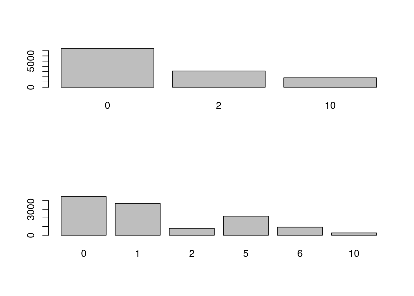

Or, a more complicated way to put them together. Here, we need to generate a table that has all of the missing values for the doubledOut. We could just enter them by hand, but then we would have to do that again. Instead, we can pull all the levels from twoTrialOut and use them.

toPlot <- rbind( table( factor(doubledOut,
                               levels = levels(factor(twoTrialOut)))
                      ),
                 table(twoTrialOut))
# See the table
toPlot

##         0    1    2    5   6   10
## [1,] 7419    0 3120    0   0 1806
## [2,] 4473 3674  795 2202 935  266

# Plot it
barplot(toPlot, beside = TRUE,
        legend.text = c("doubled","independent"))