An introduction to statistics in R
A series of tutorials by Mark Peterson for working in R
Chapter Navigation
- Basics of Data in R
- Plotting and evaluating one categorical variable
- Plotting and evaluating two categorical variables
- Analyzing shape and center of one quantitative variable
- Analyzing the spread of one quantitative variable
- Relationships between quantitative and categorical data
- Relationships between two quantitative variables
- Final Thoughts on linear regression
- A bit off topic - functions, grep, and colors
- Sampling and Loops
- Confidence Intervals
- Bootstrapping
- More on Bootstrapping
- Hypothesis testing and p-values
- Differences in proportions and statistical thresholds
- Hypothesis testing for means
- Final thoughts on hypothesis testing
- Approximating with a distribution model
- Using the normal model in practice
- Approximating for a single proportion
- Null distribution for a single proportion and limitations
- Approximating for a single mean
- CI and hypothesis tests for a single mean
- Approximating a difference in proportions
- Hypothesis test for a difference in proportions
- Difference in means
- Difference in means - Hypothesis testing and paired differences
- Shortcuts
- Testing categorical variables with Chi-sqare
- Testing proportions in groups
- Comparing the means of many groups
- Linear Regression
- Multiple Regression
- Basic Probability
- Random variables
- Conditional Probability
- Bayesian Analysis
Final thoughts on hypothesis testing
17.1 Load today’s data
Start by loading today’s data. If you need to download the data, you can do so from these links, Save each to your data directory, and you should be set.
- icuAdmissions.csv
- Data on patients admitted to the ICU.
- Roller_coasters.csv
- Data on the height and drop of a sample of roller coasters.
- NFLcombineData.csv
- Data on past NFL combine participants
# Set working directory
# Note: copy the path from your old script to match your directories
setwd("~/path/to/class/scripts")

# Load data
rollerCoaster <- read.csv("../data/Roller_coasters.csv")
icu           <- read.csv("../data/icuAdmissions.csv")
nflCombine    <- read.csv("../data/NFLcombineData.csv")
17.2 Overview
This chapter finalizes a few introductory thoughts on hypothesis testing and p-values. We start by closing the loop on the last type of relationship that we have been investigating, and move on to a few dangers, reminders, and warnings about interpretting p-values. The rest of these chapters will rely heavily on a clear understanding of p-values, so make sure that this chapter (and the last few) make sense to you before continuing on.
17.3 Generating nulls for correlations
When generating a null distribution, we need to think about what our underlying test is actually asking about. For a correlation, the test is, essentially, asking if two variables are related to one another. So, our null distribution is no relationship between the variables, meaning that we should sample each separately, then measure their correlation value. To start, let’s look at an example with a clear relationship
Let’s dive right in. As always, first define our null an alternative hypotheses. Then, calculate the value for our sample (in this case, the roller coasters in the data set). Finally, generate random data several times to see if the value for our sample is extreme or expected given the null.
H0: Coaster drop is not related to coaster speed
Ha: Coaster drop is positively related to coaster speed
Note that here, I am specifying a one-tailed alternative because our knowledge of physics suggests a relationship. Now, let’s look at our data.
# Plot the data
plot(Speed ~ Drop, data= rollerCoaster)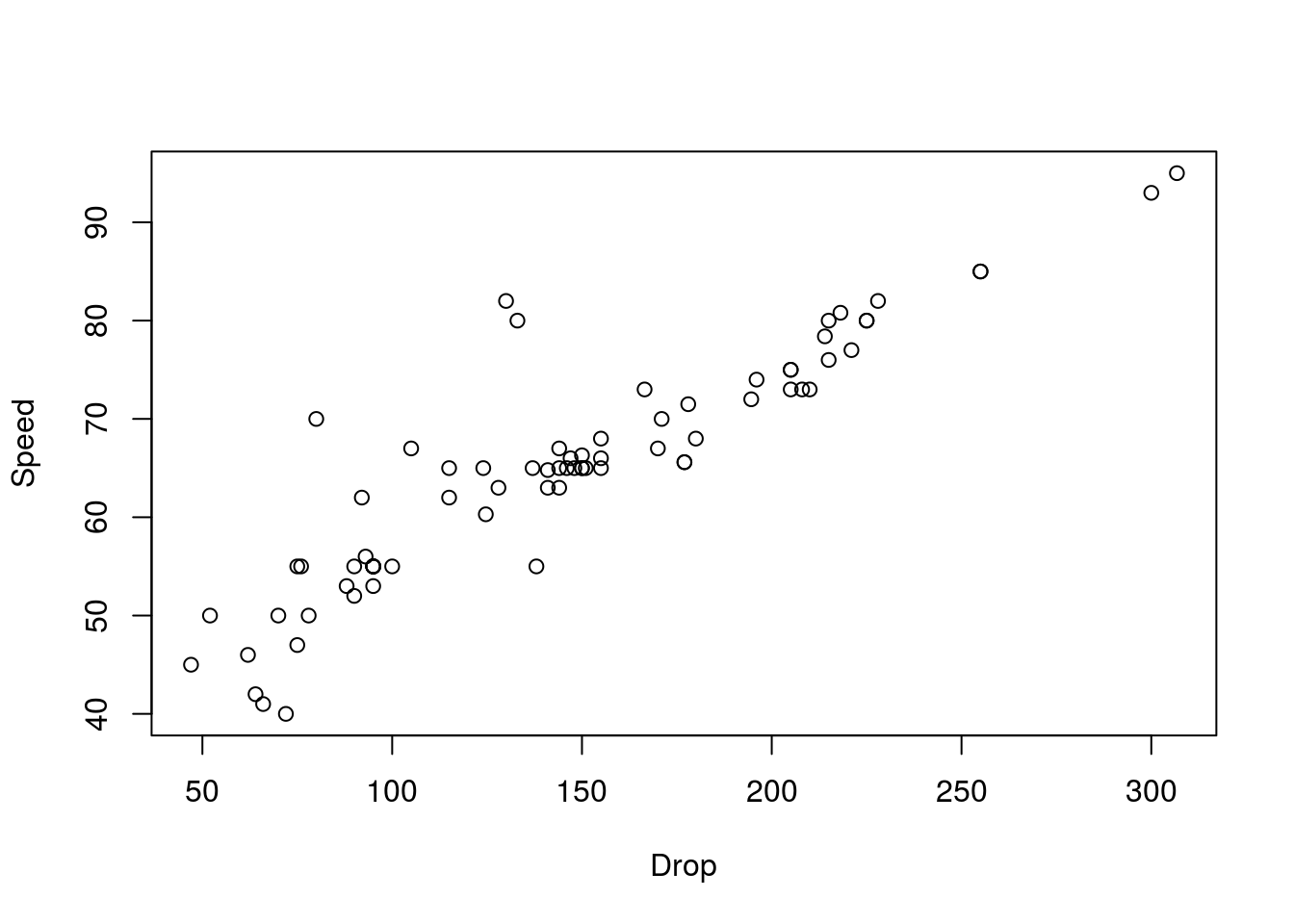
# Calculate the correlation
actualCor <- cor(rollerCoaster$Speed, rollerCoaster$Drop)
actualCor
## [1] 0.9096954Now, we need to generate data from a null distribution. To do this, we want to ask what the relationship between Speed and Drop would look like if we just randomly matched them together.
Like when randomizing for groups, we can randomize just one of the two variables because that gives us a lack of relationship (our null). We are also sampling with out replacement so that we use exactly the same values every time, just shuffled. Randomizing both or using replacement are not “wrong,” but they are are slightly different.
# Initialize variable
sampleCors <- numeric()

# Loop to create distribution
for(i in 1:13579){
  # Generate sampled data
  tempDrop <- sample(rollerCoaster$Drop)

  # Save the sample correlation
  sampleCors[i] <- cor(tempDrop, rollerCoaster$Speed)
}

# Plot the result
hist(sampleCors,
     main = "Null distribution of correlation",
     xlab = "Sample Correlation")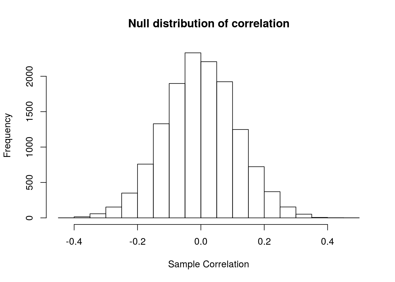
Notice that none of these values are even close to our observed correlation (r = 0.91). We can confirm this by calculating the p-value. Because we specified a one-tailed alternative, we only need to ask what proportion of values from the null are greater than our observed value.
# Calculate p value
propAsExtreme <- mean(sampleCors >= actualCor)
propAsExtreme
## [1] 0As suspected, a very tiny p-value, suggesting we definitely should reject H0.
17.3.1 Try it out
Using the icu as a sample, determine if there is a correlation between blood pressure (column Systolic) and heart rate (column HeartRate).
State your null and alternate hypotheses, build and plot a null distribution, and calculate a p-value. Make sure to interpret the p-value.
You should get a plot something like this:
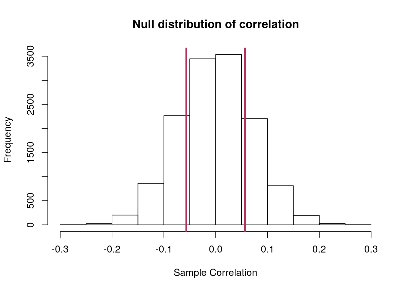
and a p-value of about 0.43. Don’t forget to interpret it.
17.4 Statistical vs. Practical Significance
In every day language, we tend to use the word “significant” rather differently than we do in statistics. We usually think of “significant” as meaning “big” or “important.” Neither of those meanings are necessarily true for statistically significant results.
Statistically significant simply implies that the results are unlikely to have occured by chance, and says nothing about about whether the result is meaningful. For example, let’s test the effects of a weight loss drug. Here, we will be creating simulated data, but the point extends to several real examples. This uses a random number generator that
we will explore more after this exam. Essentially, it will just create some unimodal, symmetric data for us with a specified mean. Note that here, we are setting the means to different values, so we expect to find a difference.
# Set seed so we all get the same data
set.seed(54601)

# Create data for people that took the drug
onPills <- rnorm(n = 100, mean = -1)

# Create data for the controls
onPlacebo <- rnorm(n = 100, mean = 0)

# Visualize the data
boxplot(onPills,onPlacebo,
        names = c("on Pills","Placebo"),
        ylab = "Weight Change (lbs)")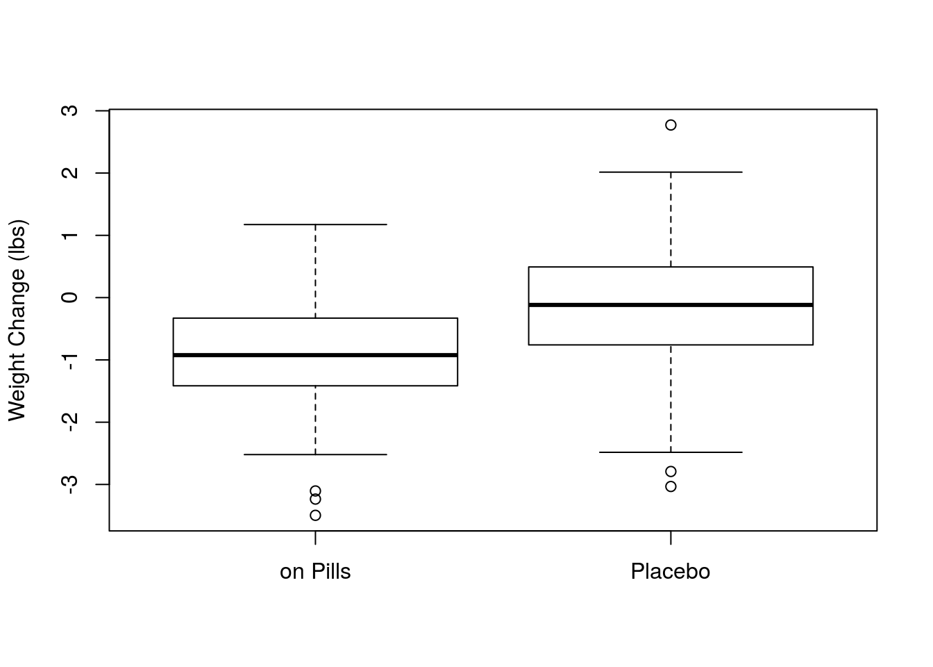
# See the difference
diffMean <- mean(onPills) - mean(onPlacebo)
diffMean
## [1] -0.7933195So, we can see that the mean weight change was more negative (by about 0.8 pounds) for those one the pills. Let’s run a quick simulation to see if that difference is statistically significant. This is largely copied from earlier examples.
# Create our pool
poolWeight <- c(onPills,onPlacebo)

# Initialize variable
sampleDiffs <- numeric()

# Run a loop to test for difference
for(i in 1:12345){
  # Create our temporary samples
  tempOnPills   <- sample(poolWeight,
                          size = length(onPills),
                          replace = TRUE)
  tempOnPlacebo <- sample(poolWeight,
                          size = length(onPlacebo),
                          replace = TRUE)

  # Store the difference
  sampleDiffs[i] <- mean(tempOnPills) - mean(tempOnPlacebo)

}


# Plot the distribution
hist(sampleDiffs)
# Add a line to show where our calculated mean falls
abline(v = c(diffMean,-diffMean), col = "red3",lwd=3)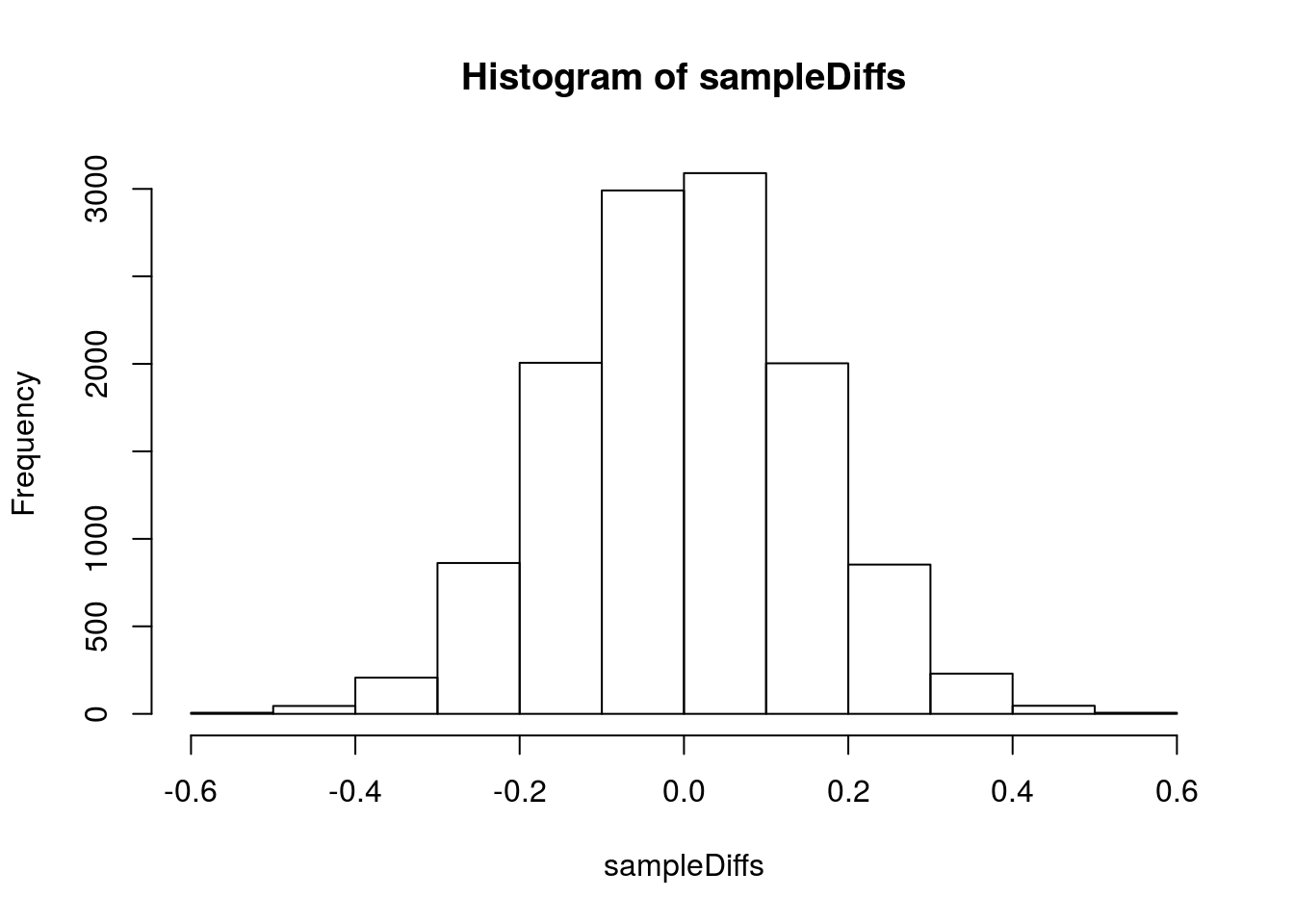
# Calculate the p-value
mean( sampleDiffs >=  abs(diffMean) |
      sampleDiffs <= -abs(diffMean)  )
## [1] 0So, we can see that the difference is very significant, and we can reject the H0 of no effect of the pills. However, is this difference meaningful? What if I told you that the study lasted one year and that the pills cost $1,000 for the year? Would the effect (a 0.8 pound weight loss) be of practical importance?
Probably not. Be wary of this conflation of statistical significance and practical significance.
17.5 Multiple Testing
Using the icu data as a sample, is the mean patient ID number (column ID) different between “elective” and “emergency” visits (column Type)? Refer back to your notes from last chapter as needed.
State your null and alternate hypotheses, build and plot a null distribution, and calculate a p-value. Make sure to interpret the p-value. Because this seems like a minor issue, use an α threshold of 0.10 (reject H0 if your p-value is less than 0.10).
You should get a plot something like this.
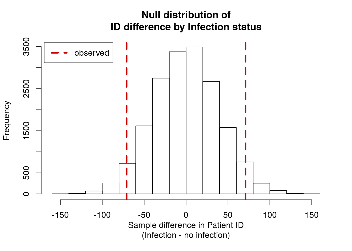
and should get a p-value of around 0.065. What can you conclude about that p-value?
It is quite small, so you are able to reject the H0 that there is no difference between ID numbers in patients with and without infections. Said another way, we have shown here that we expect patients with an infection to have a different mean ID number. However, does that make sense?
…
If ID numbers are assigned as patients arrive, do we have any reason to suspsect such a difference? I would wager that we don’t. However, there are 17 columns with factors in them. By chance, we expect some of them (about 1 in 15) to have a p-value this low or lower if the null is true. That is, the p-value we calculated (0.065) means that data that extreme (or more extreme) will only happen about 7 times in 100 trials.
How do you think I selected this column for this example? In fact, I tested every single one of the 17 factor columns and selected the one that gave me close to a significant result. This is an issue called multiple testing and it is an additional major concern for null hypothesis significance testing.
Recall that a p-value measures the probablity of generating your data (or more extreme) given that the null hypothesis is true. If we set our significance threshold (α) at 0.05, that means that we will incorrectly reject our null hypothesis roughly 1 time in 20.
This may not seem like much of an issue, as this reflects the balance we struck between Type I and Type II error. However, once we start testing multiple things, the situation changes. Imagine running 20 tests in which the null hypothesis is true. How many of them do you expect to get a p-value of less than 0.05? What if you run 200 tests?
My research generally involves testing (at least) 20,000 things all at the same time. How many of those tests do you expect should give a “significant” p-value, even if all of the null hypotheses are true[*](Answers: 1, 10, 1000.)?
This issue is crucial to understand, but correcting for it, unfortunately, falls outside the scope of this course. We will touch on it again throughout these chapters, but for now it is enough to understand and appreciate that it is an issue, without worrying about how to fix it.
To illustrate this, below is a loop of loops to test for differences between randomly drawn NFL position players. Imagine it being a series of pairwise tests between different subsets, such as kickers vs. running backs, or DI players vs. DIII players.
You DO NOT need to be able to do this, or even understand all of it. It is purely here to illustrate this phenomenon. Note that this loop takes a very long time to run, as it is doing one of our longer loops 1000 times.
# Set up an arbitrary group
groups <- rep(c("A","B"),
              c( 20, 30))

# Initialize variable to hold p-values
myPvals <- numeric()

# Loop through many tests
# usigng "k" because "i" is used in the loop inside this loop
for(k in 1:1000){
  # Copy in the sampling from the NFL Weight example

  # Get a subset of skill players
  sampleWeights <- sample(nflCombine$Weight[nflCombine$positionType == "skill"],
                          size = length(groups)
                          )

  # Quantify
  tempMeans <- by(sampleWeights, groups, mean)

  # Store the parameter of interest (the difference in means here)
  diffMean <- tempMeans["A"] - tempMeans["B"]

  # Initialize variable
  sampleDiffs <- numeric()

  # Run a loop to test for difference
  for(i in 1:10123){
    # Create our temporary samples
    reSampleWeights <- sample(sampleWeights,
                              size = length(groups),
                              replace = TRUE
                              )

    # Quantify
    veryTempMeans <- by(reSampleWeights, groups, mean)

    # Store the parameter of interest (the difference in means here)
    sampleDiffs[i] <- veryTempMeans["A"] - veryTempMeans["B"]

  }


  # Caclulate the p-value
  myPvals[k] <- mean( sampleDiffs >=  abs(diffMean) |
                      sampleDiffs <= -abs(diffMean) )

}

# Visualize p vals
hist(myPvals)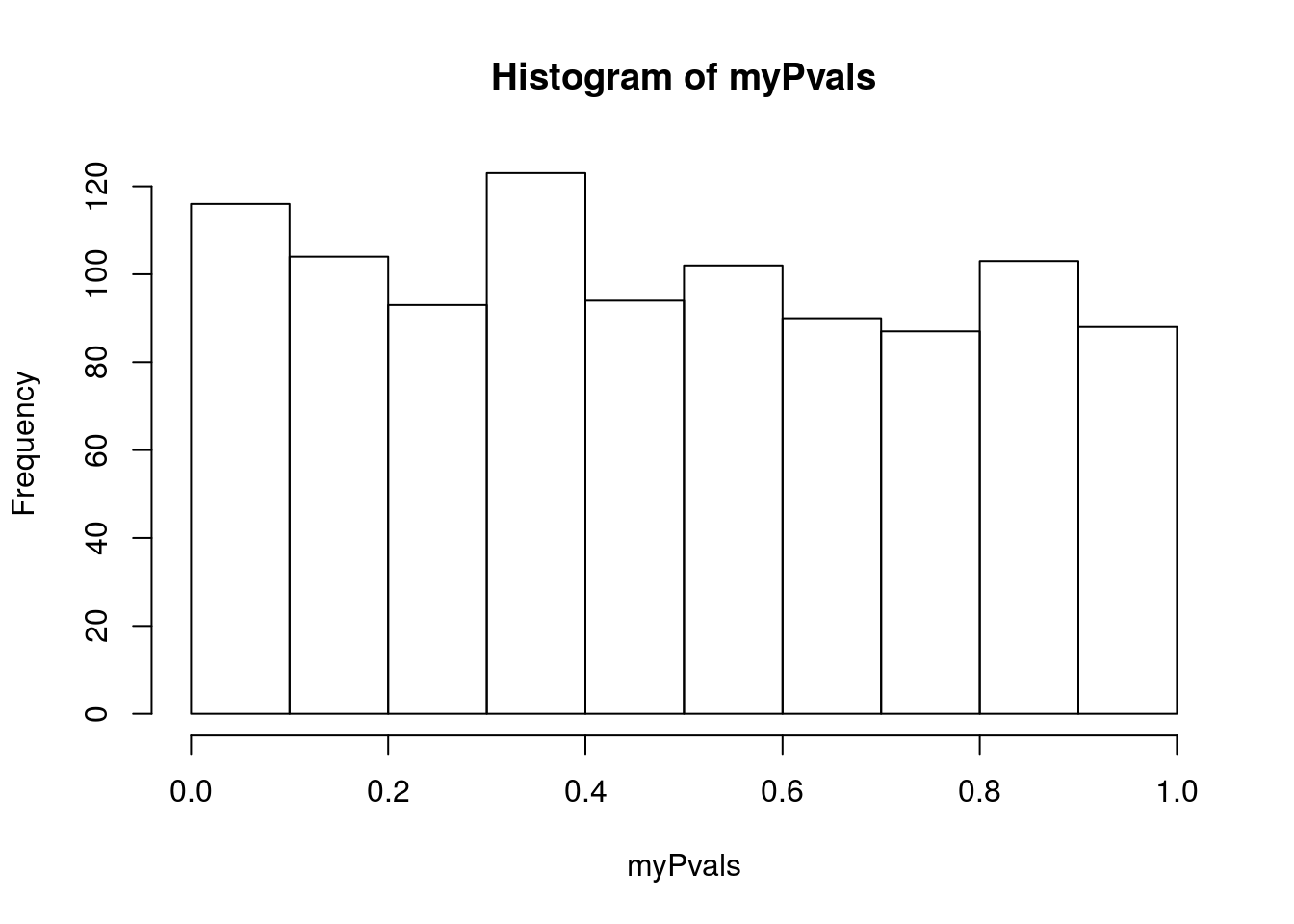
# See how many were significant
sum(myPvals < 0.05)
## [1] 59# See what proportion were significant
mean(myPvals < 0.05)## [1] 0.059As you can see, right around 5% of them were signficant even though the groups were completely arbitrary. Importatnly, that is exactly what we expect it to be as well.
As a reminder to be vigilant of this (and other issues) when reading popular reporting about science, I leave you with this excellent xkcd comic:
