33.1 Load today’s data

Start by loading today’s data. If you need to download the data, you can do so from these links, Save each to your data directory, and you should be set.

• carSalesPrice.csv
  • Kuiper, Shonda. (2008). Introduction to Multiple Regression: How Much Is Your Car Worth? Journal of Statistics Education. Volume 16, Number 3.
  • describes the relationship between the Price of 804 used 2005 GM cars and various features of the cars.
• wages1985.csv
  • Downloaded from: http://lib.stat.cmu.edu/datasets/CPS_85_Wages
  • Originally published in: Berndt, ER. The Practice of Econometrics. 1991. NY: Addison-Wesley.
  • Data originally from: the Current Population Survey of 1985
  • Gives wages (in dollars per hour) along with other demographic information for 534 individuals surveyed in 1985
    • south tells whether or not the person lives in the south
    • education gives the number of years of education
    • other columns should be self explanatory

We also want to make sure that we load any packages we know we will want near the top here.

# Set working directory
# Note: copy the path from your old script to match your directories
setwd("~/path/to/class/scripts")

# Load needed libraries
library(RColorBrewer)

# Load data
cars <- read.csv( "../data/carSalesPrice.csv" )
wages <- read.csv("../data/wages1985.csv")

33.2 Overview

Often, a simple model is not enough. We may have more information, and we want to be able to use it. In the roller coaster data, could we explain the Speed even better if we included information about the type of track (wood vs. metal)? Today, we will walk through an example implementing this, and, in doing so, touch on many of the key concepts from throughout chapter 10.

The data set we are using today comes from:

Let’s look at the data briefly to see what is there.

# Look at data
head(cars)

Price	Mileage	Make	Model	Trim	Type	Cylinder	Liter	Doors	Cruise	Sound	Leather
17314.10	8221	Buick	Century	Sedan 4D	Sedan	6	3.1	4	yes	yes	yes
17542.04	9135	Buick	Century	Sedan 4D	Sedan	6	3.1	4	yes	yes	no
16218.85	13196	Buick	Century	Sedan 4D	Sedan	6	3.1	4	yes	yes	no
16336.91	16342	Buick	Century	Sedan 4D	Sedan	6	3.1	4	yes	no	no
16339.17	19832	Buick	Century	Sedan 4D	Sedan	6	3.1	4	yes	no	yes
15709.05	22236	Buick	Century	Sedan 4D	Sedan	6	3.1	4	yes	yes	no

Now, let’s use it to predict the Price of other used cars.

33.3 A simple model

Which of those variable seems the most likely to have a good linear relationship with Price?

Thoughts?

I think we should start with Mileage, and since this is already written, let’s do that. In your own work, you could feel free to start elsewhere. This is the first of many times in this chapter that we will see that there is no single “right” answer when it comes to multiple regression. There are a lot of subjective decisions to make, and we will address them as they arise.

For our simple model:

# Make a simple model
simpleModel <- lm( Price ~ Mileage,
                   data = cars)

# Look at the basic output
simpleModel

## 
## Call:
## lm(formula = Price ~ Mileage, data = cars)
## 
## Coefficients:
## (Intercept)      Mileage  
##  24764.5590      -0.1725

What does this model tell us? If we write out the equation it looks like:

Price = 24764.56 + -0.17 * Mileage

So, the baseline price for a car is $24764.56 if it has been driven 0 miles, and for each mile driven it is worth $0.17 less. Does this make intuitive sense?

Does that mean that mileage doesn’t matter, since the value is so small (only a few cents)? Recall that the difference in miles driven can be thousands of dollars. So, those cents can add up quickly.

But, we probably want to know if this is significant, so let’s look at the more complete output:

# Look at summary output
summary(simpleModel)

## 
## Call:
## lm(formula = Price ~ Mileage, data = cars)
## 
## Residuals:
##    Min     1Q Median     3Q    Max 
## -13905  -7254  -3520   5188  46091 
## 
## Coefficients:
##               Estimate Std. Error t value Pr(>|t|)    
## (Intercept)  2.476e+04  9.044e+02  27.383  < 2e-16 ***
## Mileage     -1.725e-01  4.215e-02  -4.093 4.68e-05 ***
## ---
## Signif. codes:  0 '***' 0.001 '**' 0.01 '*' 0.05 '.' 0.1 ' ' 1
## 
## Residual standard error: 9789 on 802 degrees of freedom
## Multiple R-squared:  0.02046,    Adjusted R-squared:  0.01924 
## F-statistic: 16.75 on 1 and 802 DF,  p-value: 4.685e-05

Here we see that, as we expected, the effect of mileage is significant (and rather strongly so). However – let’s take a look at the R². What does that show us? Here, we have only explained 2% of the variance. How is that possible, given the significant p-value? Well, here is a case that shows how differently those two numbers operate. With large sample size, even explaining a small portion of variance can give you a signficant result.

But, it also reminds us of a step that we (intentionally in my case) skipped: plotting the data to see how it makes us feel. Let’s do that now, adding the regression line we made.

# Plot the data -- should have done this sooner
plot(Price ~ Mileage,
     data = cars)
abline(simpleModel,
       col = "red3", lwd = 3)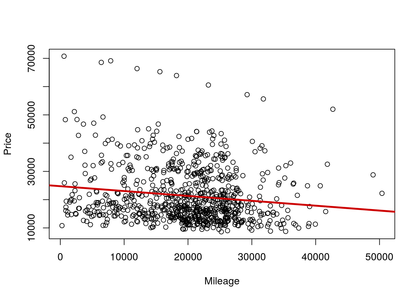

Wow – that is a lot of variation, including a set of really, really high outliers. Let’s explore that more.

33.4 A more complicated model

Among that set of outliers, there is still a (very) strong relationship with Mileage. Any guesses from the data what might cause those? Let’s look at what variables we have again.

# What variables do we have?
names(cars)

##  [1] "Price"    "Mileage"  "Make"     "Model"    "Trim"     "Type"    
##  [7] "Cylinder" "Liter"    "Doors"    "Cruise"   "Sound"    "Leather"

One that stands out (and gives us a fighting chance of visualization) is the Make of the car. Let’s see what is included there:

# What makes do we have
table(cars$Make)

## 
##     Buick  Cadillac Chevrolet   Pontiac      SAAB    Saturn 
##        80        80       320       150       114        60

Well, this certainly suggets that something might be going on. Do you think a Cadillac and a Saturn are likely to cost the same amount, given the same Mileage? Probably not. This time, before we add it to the model, let’s plot the data. Here, we are going to set the colors directly, and use some of the cool features of R to do so.

First, let’s pick some colors. I am going to use the RColorBrewer package that we have talked about, but also show you how to do it yourself, if you prefer (or don’t have that package)

# how many colors do we need?
nColors <- length(levels(cars$Make))
nColors

## [1] 6

# Use the builtin palette
myColors <- palette()[1:nColors]


# OR: By hand
myColors <- c("red3","brown","green3",
              "darkblue","orange","purple")

# OR: Use RColorBrewer
# Try  display.brewer.all() to see more options
myColors <- brewer.pal(nColors, "Set1")

Now, we can create a new variable to hold our colors, and just change the names to match the colors we want.

# Create color variable
cars$makeColor <- cars$Make

# Change names
levels(cars$makeColor) <- myColors

# Display table
table(cars$makeColor,cars$Make)

	Buick	Cadillac	Chevrolet	Pontiac	SAAB	Saturn
#E41A1C	80	0	0	0	0	0
#377EB8	0	80	0	0	0	0
#4DAF4A	0	0	320	0	0	0
#984EA3	0	0	0	150	0	0
#FF7F00	0	0	0	0	114	0
#FFFF33	0	0	0	0	0	60

Note that the order of the colors matches that from the makes. So, we now have a color matched up to each make. For more variables than this (like if we started with Model), this would not be possible to do without being very messy. Now, lets plot this again.

A few notes. The as.character() is neccesary because cars$makeColor is a factor, and thus will be treated as numeric variable without as.character() (yielding the ugly default palette() colors instead of the colors you picked). I added the argument pch = 19 to give solid circles, instead of open ones, as they show the colors better. The pch = agrument can take either a number, which corresponds to specific shapes (see ?pch for more info), or a character (such as a letter) to be used as the point.

# Plot with colors
plot(Price ~ Mileage,
     data = cars,
     pch = 19,
     col = as.character(cars$makeColor)  )

# Add legend
legend( "topright", inset = 0.01,
        legend = levels(cars$Make),
        pch = 19,
        col = levels(cars$makeColor))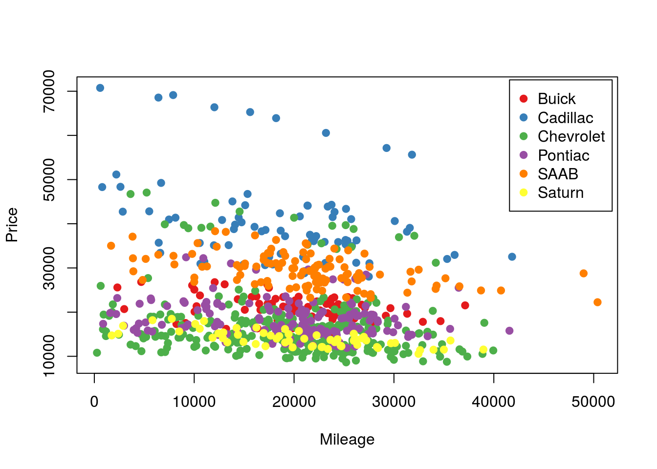

So, we can see now that there is a clear stratificiation by Make. Are you surprised to see Cadillac consistently near the top or Saturn consistently near the bottom? (There is more stratification that we will handle shortly as well.) For now, let’s add make to our model. It is as simple as writing the equation we are interested in.

# Create the model
modelWithMake <- lm( Price ~ Make + Mileage,
                     data = cars)

# View simple version
modelWithMake

## 
## Call:
## lm(formula = Price ~ Make + Mileage, data = cars)
## 
## Coefficients:
##   (Intercept)   MakeCadillac  MakeChevrolet    MakePontiac       MakeSAAB  
##    24305.9186     19861.5592     -4519.5234     -2592.2556      8771.1877  
##    MakeSaturn        Mileage  
##    -6852.0873        -0.1709

So, our equation still has Mileage at about -17 cents per mile, but now adds some changes to the intercept. Here, Buick is our “reference” meaning the “intercept” reported gives us the predicted Price of a Buick with 0 miles on it. For each additional Make, R is telling us how much to adjust the price for a car with no miles on it. For Cadillace we need to add $20k! For a Saturn, we subtract almost $7k. The slope for each is still the same, -$0.17 for each mile driven.

We can add those lines to the plot, though abline() can no longer do it directly. There are lots of ways to do it, though here, I am going to use a for() loop and curve(). Each time through the loop, I am going to use our index (here k) to make a line from the predict values for that Make, and using our saved color that matches. By setting Make as a single variable, it is repeated as many times as curve needs.

# Make the base plot (you probably don't need to rerun this)
# Plot with colors
plot(Price ~ Mileage,
     data = cars,
     pch = 19,
     col = as.character(cars$makeColor)  )

# Add legend
legend( "topright", inset = 0.01,
        legend = levels(cars$Make),
        pch = 19,
        col = levels(cars$makeColor))

# Add lines
# Loop through the makes and colors
for( k in 1:length(levels(cars$Make)) ){
  curve( predict( modelWithMake,
                  data.frame( Make = levels(cars$Make)[k],
                              Mileage= x)),
         col = levels(cars$makeColor)[k],
         lwd = 3,
         add = TRUE)
  
}

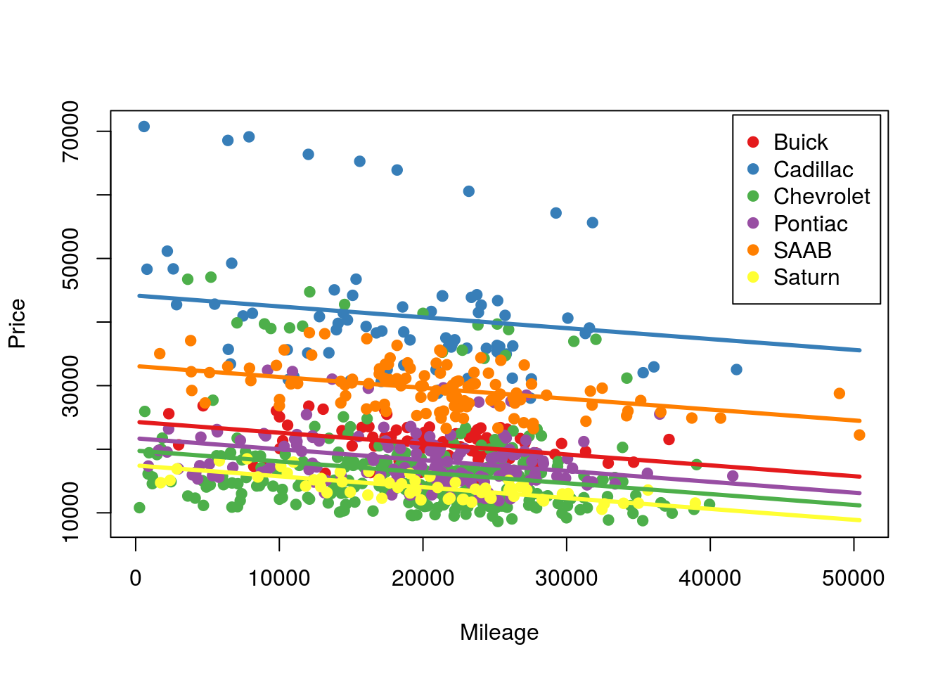
Here, we now see that we have 6 parallel lines – one for each model. All that adding the Make to the model did is move the intercept, so for each Make, we see that the mileage causes a similar reduction in Price – but from a different starting point.

Let’s take a look at the details of the model to see what else we can say:

# Look at model details
summary(modelWithMake)

## 
## Call:
## lm(formula = Price ~ Make + Mileage, data = cars)
## 
## Residuals:
##      Min       1Q   Median       3Q      Max 
## -11755.2  -3274.0   -701.8   1517.1  28174.1 
## 
## Coefficients:
##                 Estimate Std. Error t value Pr(>|t|)    
## (Intercept)    2.431e+04  8.182e+02  29.705  < 2e-16 ***
## MakeCadillac   1.986e+04  9.093e+02  21.844  < 2e-16 ***
## MakeChevrolet -4.520e+03  7.185e+02  -6.290 5.22e-10 ***
## MakePontiac   -2.592e+03  7.959e+02  -3.257  0.00117 ** 
## MakeSAAB       8.771e+03  8.381e+02  10.465  < 2e-16 ***
## MakeSaturn    -6.852e+03  9.813e+02  -6.983 6.10e-12 ***
## Mileage       -1.709e-01  2.481e-02  -6.888 1.15e-11 ***
## ---
## Signif. codes:  0 '***' 0.001 '**' 0.01 '*' 0.05 '.' 0.1 ' ' 1
## 
## Residual standard error: 5746 on 797 degrees of freedom
## Multiple R-squared:  0.6647, Adjusted R-squared:  0.6621 
## F-statistic: 263.3 on 6 and 797 DF,  p-value: < 2.2e-16

So, our model p-vale is now even smaller than before, and our R² has jumped all the way up to explaining 66.47% of the variance.

Finally, we should check the residuals to see if the meet our assumptions.

# Plot residual histogram
hist( resid(modelWithMake))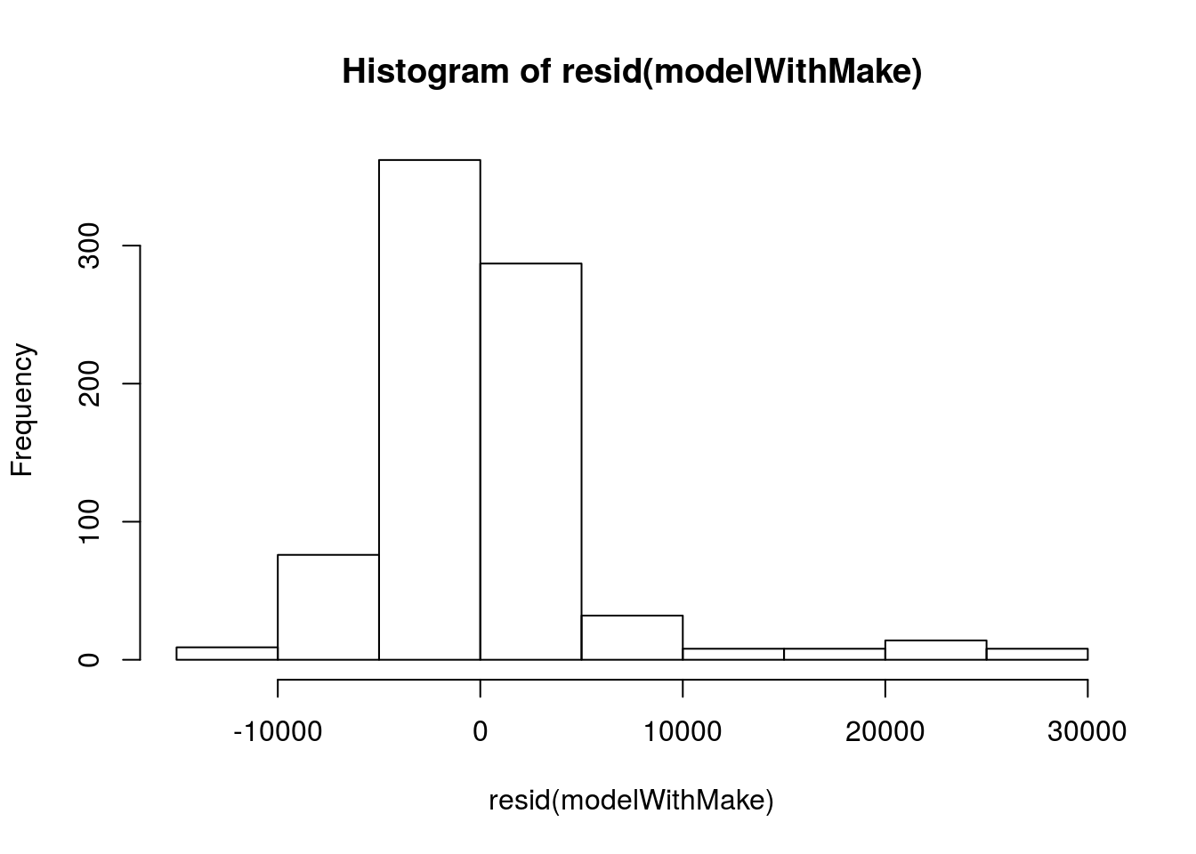

This looks like there are some larger outliers, likely those very high priced cars. We should probably try to address those before we the end of today, but they aren’t too bad for now.

# Plot resid vs predicted
plot( resid(modelWithMake) ~ predict(modelWithMake))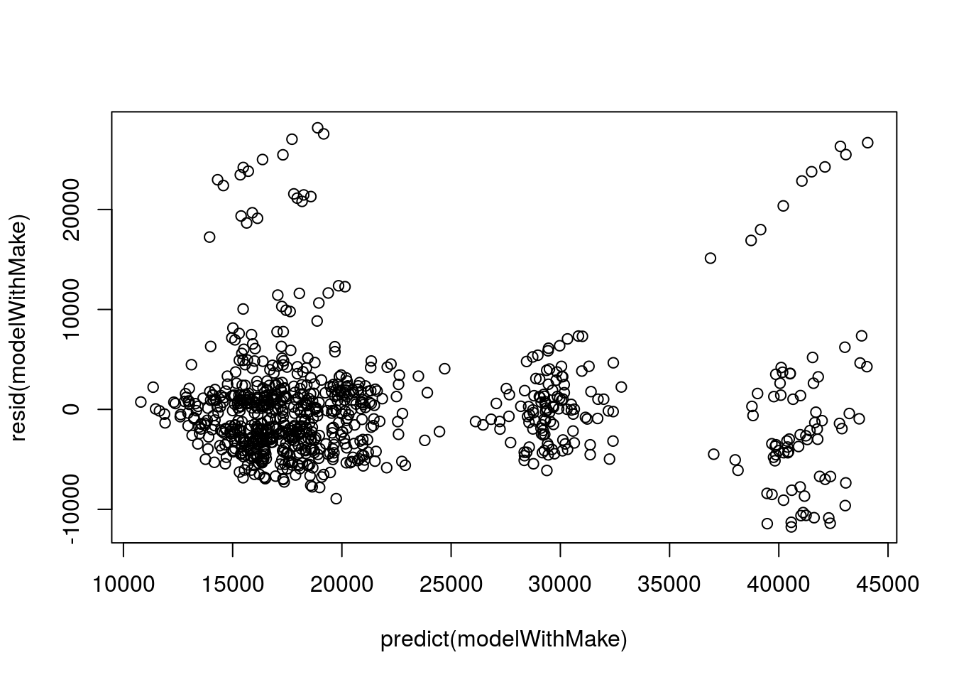

Here we see those outliers again, here showing a postive trend. These are problematic. If we continue with this model, we will need to address them.

33.5 Adding a continuous predictor

The above model is great, but it only applies to these 6 GM Makes. Does it tell us anything about how much a Ford might cost? Instead of relying on the Make, let’s see what we can do by adding additional variables. From our set of variables, what other numeric variables are likely to play a role?

# look at variables again
names(cars)

##  [1] "Price"     "Mileage"   "Make"      "Model"     "Trim"     
##  [6] "Type"      "Cylinder"  "Liter"     "Doors"     "Cruise"   
## [11] "Sound"     "Leather"   "makeColor"

Let’s try using a measure of engine size. The variable Liter gives us the volume of the engine in liters. Unfortunately, we now lose the ability to easily plot these interactions. There are some approaches, but they are rather more complicated than we have time for today. Let’s add Liter it the model and see what we get.

# Make model with engine size
modelEngSize <- lm( Price ~ Mileage + Liter,
                    data = cars)

# View simple
modelEngSize

## 
## Call:
## lm(formula = Price ~ Mileage + Liter, data = cars)
## 
## Coefficients:
## (Intercept)      Mileage        Liter  
##     9426.60        -0.16      4968.28

Here, our interpretation is a little bit different. Instead of changing the intercept, this means that we have a second slope affecting our model. So, our Intercept of $9427 if it has been driven 0 miles and has an engine of 0 Liters. Does that make sense? No, but we still need a starting point. The model then says that for each mile driven a car is worth $0.16 less, if we hold the engine size constant (and, we don’t expect the engine size to change as we drive a car). Finally, it says that, for a given number of miles driven, a car with an engine that is one liter bigger is worth $4968.28 more.

We can see this in action either by plugging things directly into the model, or by using predict().

# See the effect of changing Mileage
predict( modelEngSize,
         data.frame( Mileage = c(10000, 20000),
                     Liter =   c(  3.1,   3.1)))

##        1        2 
## 23227.98 21627.69

# See the effect of changing Liter
predict( modelEngSize,
         data.frame( Mileage = c(10000, 10000),
                     Liter =   c(  3.1,   4.1)))

##        1        2 
## 23227.98 28196.26

Let’s check the details.

# details
summary(modelEngSize)

## 
## Call:
## lm(formula = Price ~ Mileage + Liter, data = cars)
## 
## Residuals:
##    Min     1Q Median     3Q    Max 
##  -8817  -4990  -3337   3041  38568 
## 
## Coefficients:
##               Estimate Std. Error t value Pr(>|t|)    
## (Intercept) 9426.60147 1095.07777   8.608  < 2e-16 ***
## Mileage       -0.16003    0.03491  -4.584 5.28e-06 ***
## Liter       4968.27812  258.80114  19.197  < 2e-16 ***
## ---
## Signif. codes:  0 '***' 0.001 '**' 0.01 '*' 0.05 '.' 0.1 ' ' 1
## 
## Residual standard error: 8106 on 801 degrees of freedom
## Multiple R-squared:  0.3291, Adjusted R-squared:  0.3275 
## F-statistic: 196.5 on 2 and 801 DF,  p-value: < 2.2e-16

Here, we are only explaining 33% of the varianace, though it is very significant. Knowing just this, we could guess at the price of a different used car, and get closer than if we didn’t have this information.

As always, we need to check the residuals.

# histogram of residuals
hist( resid(modelEngSize) )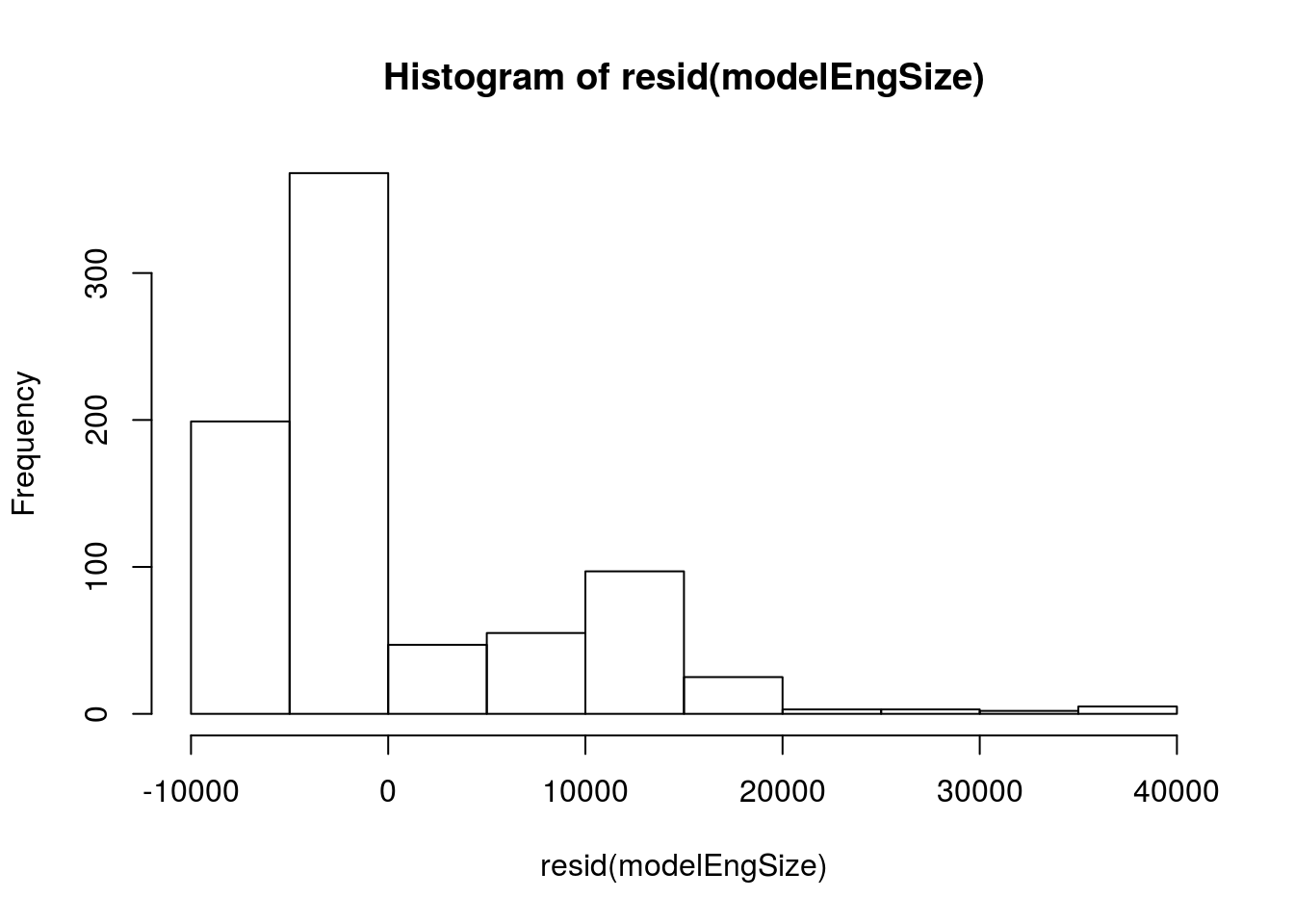

Yowzers. That is incredibly skewed. this model may give us a hint of what is going on, but it definitely doesn’t follow the assumptions we have talked about. We should be very careful with these data, and might want to consider a transformation (something beyond the scope of this class).

# Resid vs. predicted
plot( resid(modelEngSize) ~ predict(modelEngSize) )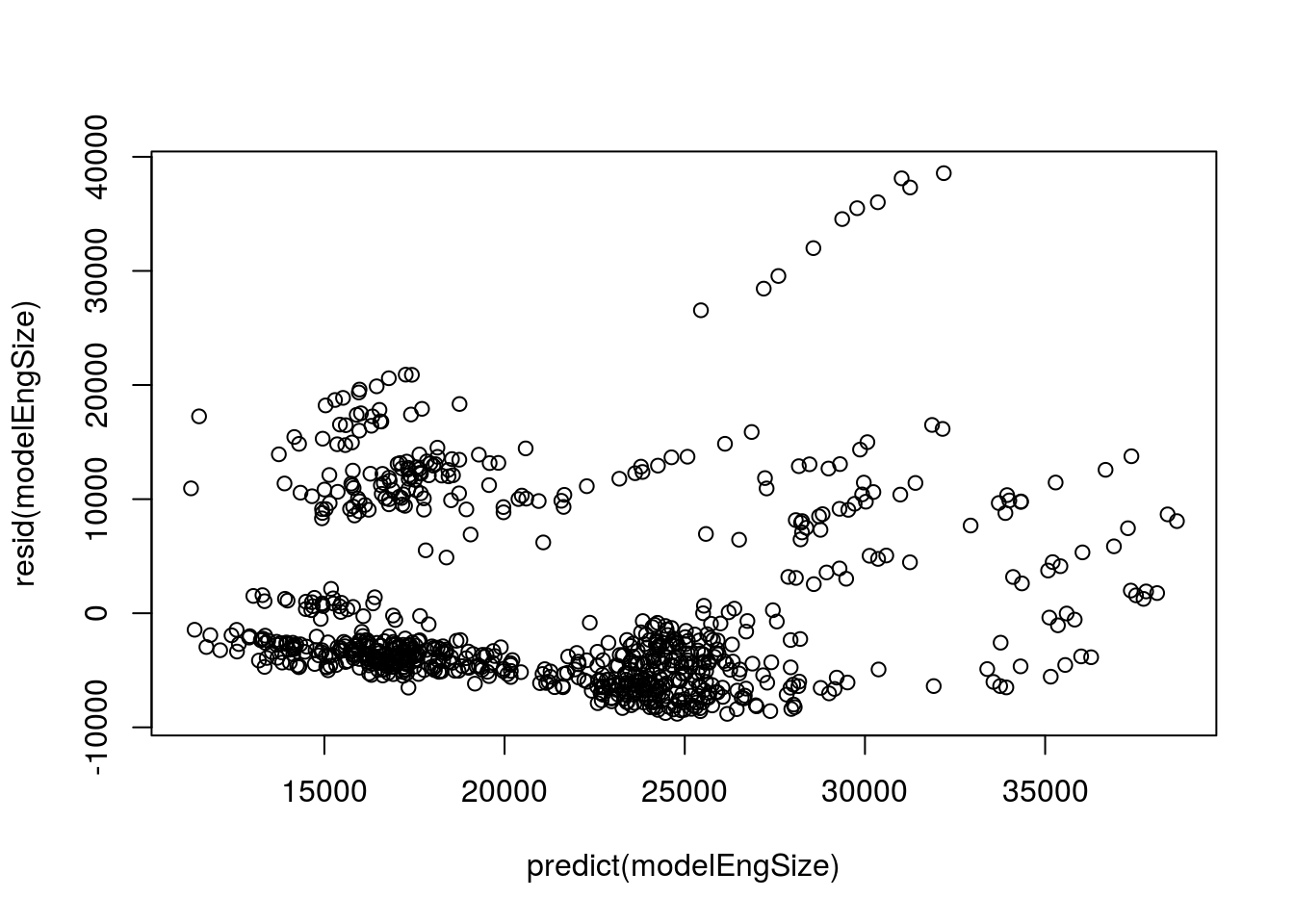

While we can’t plot the raw data easily, we can look at the residuals against the predicted values. Here, we once again see some very clear patterns. there is something wrong with this model. Below we will try to fix it a little bit, but we won’t quite make it.

33.6 Combine Categorical and numeric

Let’s try to fix up the model above by adding some more information. There is no limit to how many predictors we can use (though having too many makes our model less meaningful). Let’s see if the Type of car makes a difference. First, what types do we have?

# See car types
table(cars$Type)

## 
## Convertible       Coupe   Hatchback       Sedan       Wagon 
##          50         140          60         490          64

It seems like that might help explain some of what we are seeing, so let’s try adding it to the model. Note that I am using very descriptive model names, which can help us later.

# More complex model
modelWithTypeAndSize <- lm (Price ~ Mileage + Liter + Type,
                            data = cars)

# View simple
modelWithTypeAndSize

## 
## Call:
## lm(formula = Price ~ Mileage + Liter + Type, data = cars)
## 
## Coefficients:
##   (Intercept)        Mileage          Liter      TypeCoupe  TypeHatchback  
##     2.775e+04     -1.848e-01      5.092e+03     -2.240e+04     -2.304e+04  
##     TypeSedan      TypeWagon  
##    -1.914e+04     -1.167e+04

Here, we now have a base Price for a Convertible with 0 miles and a 0 liter engine. Each of the parameters tell us about their effects when everything else is constant. So, from this, we know something about the role of each variable. Let’s check the detailed output.

# Detailed output
summary(modelWithTypeAndSize)

## 
## Call:
## lm(formula = Price ~ Mileage + Liter + Type, data = cars)
## 
## Residuals:
##    Min     1Q Median     3Q    Max 
## -15697  -3817  -1651   1897  19686 
## 
## Coefficients:
##                 Estimate Std. Error t value Pr(>|t|)    
## (Intercept)    2.775e+04  1.218e+03  22.789  < 2e-16 ***
## Mileage       -1.848e-01  2.605e-02  -7.097 2.82e-12 ***
## Liter          5.092e+03  2.020e+02  25.210  < 2e-16 ***
## TypeCoupe     -2.240e+04  9.963e+02 -22.478  < 2e-16 ***
## TypeHatchback -2.304e+04  1.168e+03 -19.720  < 2e-16 ***
## TypeSedan     -1.914e+04  8.980e+02 -21.309  < 2e-16 ***
## TypeWagon     -1.167e+04  1.168e+03  -9.994  < 2e-16 ***
## ---
## Signif. codes:  0 '***' 0.001 '**' 0.01 '*' 0.05 '.' 0.1 ' ' 1
## 
## Residual standard error: 6042 on 797 degrees of freedom
## Multiple R-squared:  0.6291, Adjusted R-squared:  0.6263 
## F-statistic: 225.3 on 6 and 797 DF,  p-value: < 2.2e-16

We are now explaining almost 63% of the variance, which is almost as much as when accounting for Make. So, this model may be nearly as good as the Make approach, but is applicable to other types of cars as well.

Finally, as always, we need to check the residuals.

# Histogram
hist( resid(modelWithTypeAndSize) )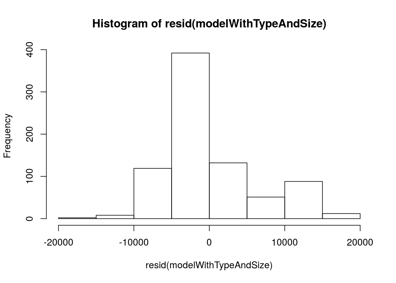

This certainly looks a lot more normal. What about the relationship with predicted?

# Plot vs predicted
plot( resid(modelWithTypeAndSize)  ~
        predict(modelWithTypeAndSize) )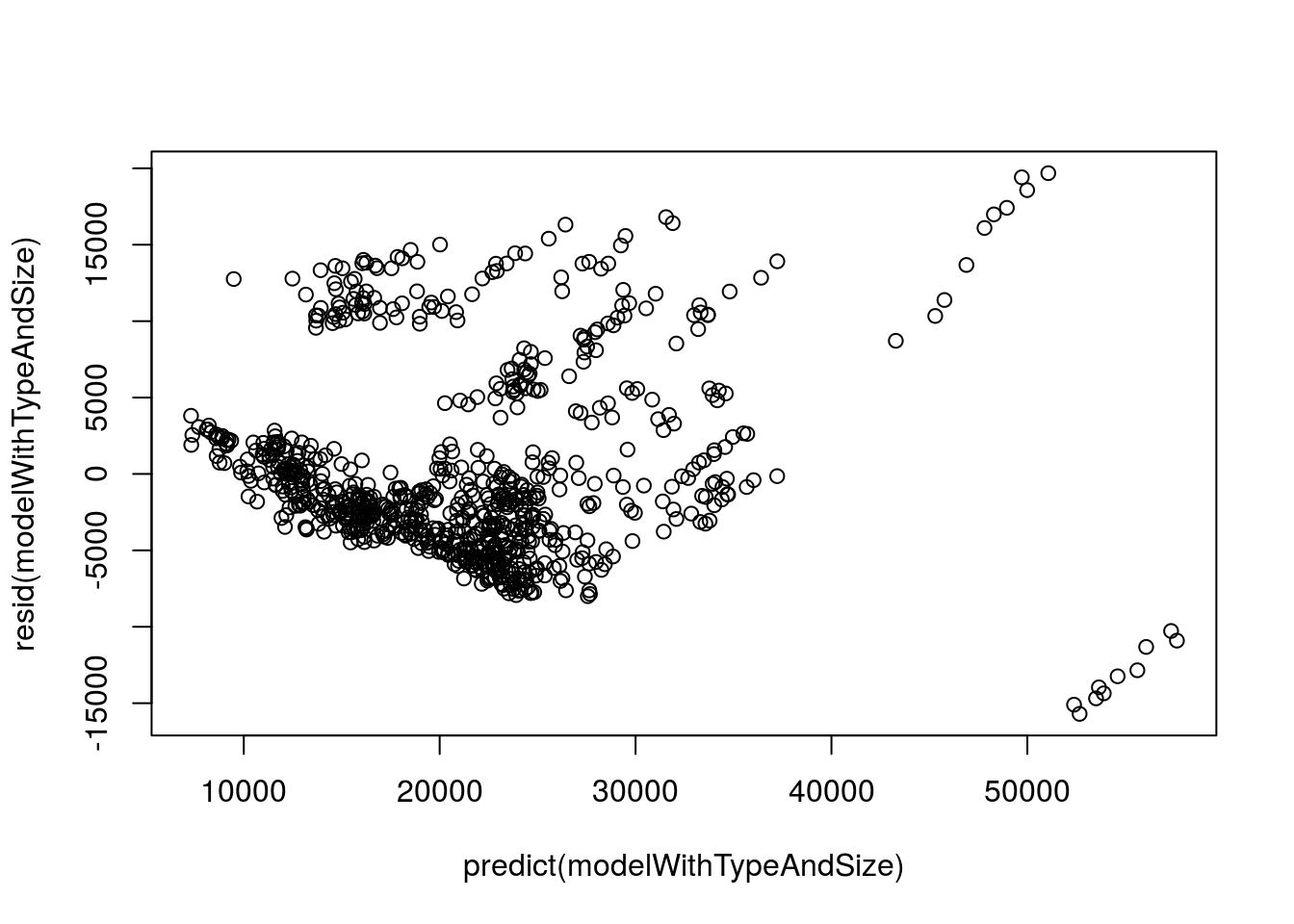

Here, we again see some clear patterns, including a hint that the relationship may not be linear (it looks like there are some curves there) and that there are still some outlying groups. We likely wouldn’t trust this model very far, but fixing up these last steps is just a bit too much for this class.

33.7 A great final model

Finally, here is a model that is great, but won’t work for any other cars. It uses the model of the car along with the mileage.

## Make the model
greatMod <- lm( Price ~ Model + Mileage,
                data = cars)

greatMod

## 
## Call:
## lm(formula = Price ~ Model + Mileage, data = cars)
## 
## Coefficients:
##      (Intercept)          Model9_3       Model9_3 HO          Model9_5  
##        2.794e+04         4.880e+03         5.999e+03         5.703e+03  
##      Model9_5 HO         ModelAVEO   ModelBonneville     ModelCavalier  
##        4.035e+03        -1.373e+04        -3.618e+03        -1.165e+04  
##     ModelCentury      ModelClassic       ModelCobalt     ModelCorvette  
##       -8.746e+03        -1.076e+04        -1.067e+04         1.440e+04  
##       ModelCST-V          ModelCTS      ModelDeville           ModelG6  
##        2.042e+04         5.381e+03         1.171e+04        -4.881e+03  
##    ModelGrand Am   ModelGrand Prix          ModelGTO       ModelImpala  
##       -1.012e+04        -6.392e+03         4.812e+03        -4.485e+03  
##         ModelIon     ModelLacrosse      ModelLesabre     ModelL Series  
##       -1.084e+04        -3.195e+03        -4.587e+03        -8.520e+03  
##      ModelMalibu  ModelMonte Carlo  ModelPark Avenue       ModelSTS-V6  
##       -7.484e+03        -4.639e+03        -6.569e+02         1.268e+04  
##      ModelSTS-V8      ModelSunfire         ModelVibe       ModelXLR-V8  
##        1.822e+04        -1.171e+04        -8.668e+03         3.823e+04  
##          Mileage  
##       -1.724e-01

Here, we see that every Model of car has it’s own intercept, but that they share a slope. This makes intuitive sense as it shows us what we probably thought already. This is a great model if you want to know the Price of one of these particular cars … but not such a great model if you are interested in the price of a different type of car (e.g. Ford). That balance, along with several other factors, is important to consider when selecting models. The particulars will depend the exact nature of your question.

For completeness, let’s look at the details of the full model. First, let’s see the ANOVA output, as that will give us a single value for significance of the Models in the model.

# Look at ANOVA output
anova(greatMod)

## Analysis of Variance Table
## 
## Response: Price
##            Df     Sum Sq    Mean Sq F value    Pr(>F)    
## Model      31 7.4457e+10 2401848775  753.82 < 2.2e-16 ***
## Mileage     1 1.5475e+09 1547488052  485.68 < 2.2e-16 ***
## Residuals 771 2.4566e+09    3186229                      
## ---
## Signif. codes:  0 '***' 0.001 '**' 0.01 '*' 0.05 '.' 0.1 ' ' 1

So, everything is incredibly significant, and the Model accounts for a HUGE portion of the variance in the model. Let’s look directly at the effects of each, along with the R² value:

# See full details
summary(greatMod)

## 
## Call:
## lm(formula = Price ~ Model + Mileage, data = cars)
## 
## Residuals:
##     Min      1Q  Median      3Q     Max 
## -6812.0  -938.3    -0.1   868.1  6497.9 
## 
## Coefficients:
##                    Estimate Std. Error t value Pr(>|t|)    
## (Intercept)       2.794e+04  9.027e+02  30.952  < 2e-16 ***
## Model9_3          4.880e+03  9.783e+02   4.988 7.55e-07 ***
## Model9_3 HO       5.999e+03  9.364e+02   6.407 2.58e-10 ***
## Model9_5          5.703e+03  9.506e+02   5.999 3.05e-09 ***
## Model9_5 HO       4.035e+03  9.784e+02   4.125 4.12e-05 ***
## ModelAVEO        -1.373e+04  9.220e+02 -14.896  < 2e-16 ***
## ModelBonneville  -3.618e+03  9.504e+02  -3.807 0.000152 ***
## ModelCavalier    -1.165e+04  9.220e+02 -12.638  < 2e-16 ***
## ModelCentury     -8.746e+03  1.056e+03  -8.281 5.37e-16 ***
## ModelClassic     -1.076e+04  1.056e+03 -10.188  < 2e-16 ***
## ModelCobalt      -1.067e+04  9.276e+02 -11.507  < 2e-16 ***
## ModelCorvette     1.440e+04  9.777e+02  14.726  < 2e-16 ***
## ModelCST-V        2.042e+04  1.056e+03  19.332  < 2e-16 ***
## ModelCTS          5.381e+03  1.056e+03   5.095 4.39e-07 ***
## ModelDeville      1.171e+04  9.503e+02  12.321  < 2e-16 ***
## ModelG6          -4.881e+03  9.779e+02  -4.991 7.43e-07 ***
## ModelGrand Am    -1.012e+04  9.783e+02 -10.350  < 2e-16 ***
## ModelGrand Prix  -6.392e+03  9.506e+02  -6.724 3.45e-11 ***
## ModelGTO          4.812e+03  1.056e+03   4.555 6.08e-06 ***
## ModelImpala      -4.485e+03  9.505e+02  -4.719 2.82e-06 ***
## ModelIon         -1.084e+04  9.280e+02 -11.683  < 2e-16 ***
## ModelLacrosse    -3.195e+03  9.507e+02  -3.361 0.000815 ***
## ModelLesabre     -4.587e+03  9.783e+02  -4.689 3.25e-06 ***
## ModelL Series    -8.520e+03  1.056e+03  -8.068 2.73e-15 ***
## ModelMalibu      -7.484e+03  9.219e+02  -8.119 1.86e-15 ***
## ModelMonte Carlo -4.639e+03  9.504e+02  -4.881 1.28e-06 ***
## ModelPark Avenue -6.569e+02  9.778e+02  -0.672 0.501890    
## ModelSTS-V6       1.268e+04  1.056e+03  12.006  < 2e-16 ***
## ModelSTS-V8       1.822e+04  1.056e+03  17.250  < 2e-16 ***
## ModelSunfire     -1.171e+04  1.056e+03 -11.085  < 2e-16 ***
## ModelVibe        -8.668e+03  9.503e+02  -9.121  < 2e-16 ***
## ModelXLR-V8       3.823e+04  1.056e+03  36.204  < 2e-16 ***
## Mileage          -1.724e-01  7.823e-03 -22.038  < 2e-16 ***
## ---
## Signif. codes:  0 '***' 0.001 '**' 0.01 '*' 0.05 '.' 0.1 ' ' 1
## 
## Residual standard error: 1785 on 771 degrees of freedom
## Multiple R-squared:  0.9687, Adjusted R-squared:  0.9674 
## F-statistic: 745.4 on 32 and 771 DF,  p-value: < 2.2e-16

We can see from this that we are explaining 96.9% of the variance. To see the R² directly we can use this trick to avoid prining the entire table.

summary(greatMod)$r.squared

## [1] 0.9686905

Finally, lets plot the residuals to check things.

# Plot residuals
plot( resid(greatMod) ~ predict(greatMod) )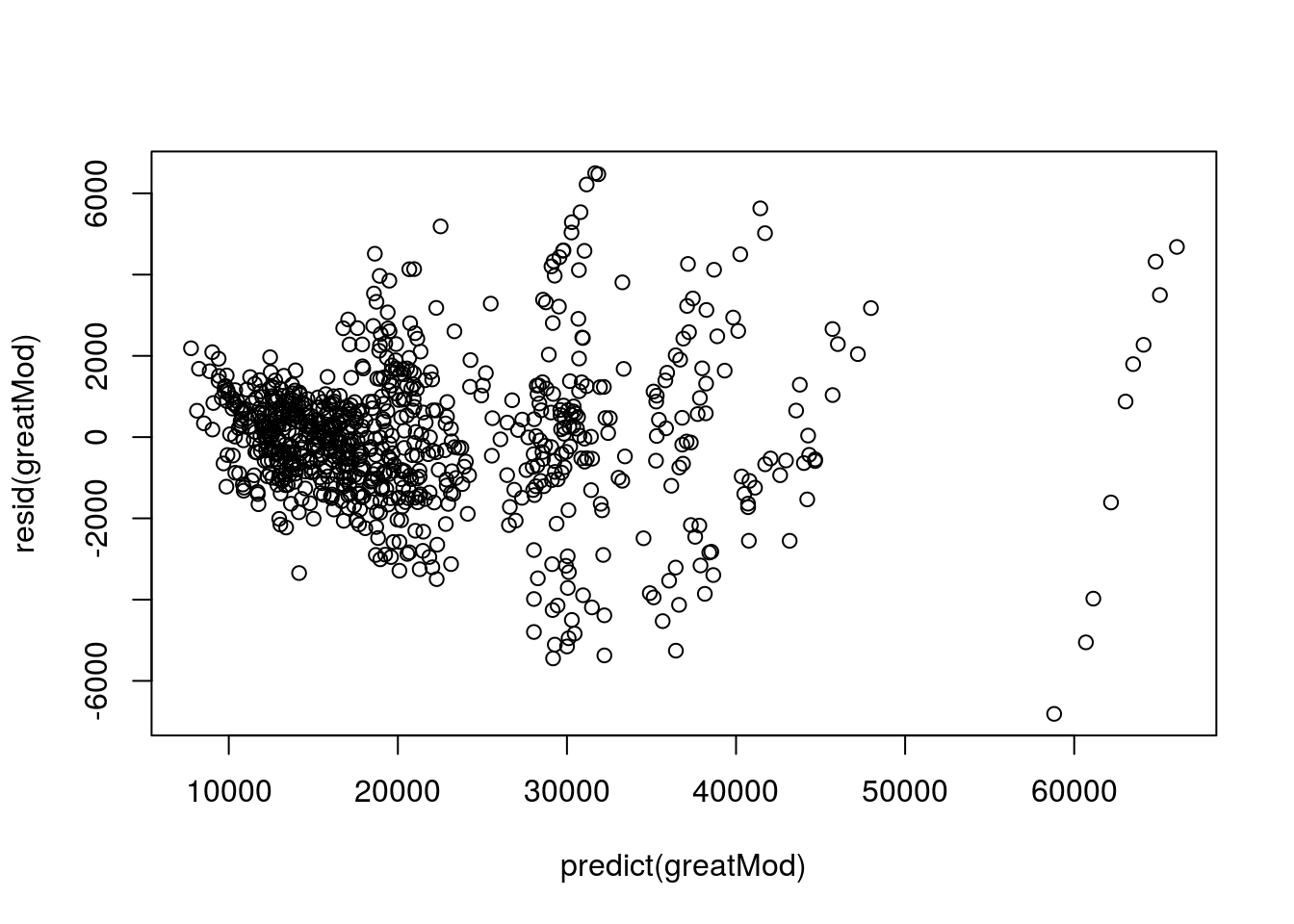

Here, we have gotten rid of most of the groups and patterns, and there is not much of a pattern. There is a slightly smaller magnitude of residuals at the very low levels, but we would probably be ok using this model to predict the price of other cars. (To fix this, we would use data transformation, but that is just a bit more complicated than I want to make this tutorial.)