An introduction to statistics in R
A series of tutorials by Mark Peterson for working in R
Chapter Navigation
- Basics of Data in R
- Plotting and evaluating one categorical variable
- Plotting and evaluating two categorical variables
- Analyzing shape and center of one quantitative variable
- Analyzing the spread of one quantitative variable
- Relationships between quantitative and categorical data
- Relationships between two quantitative variables
- Final Thoughts on linear regression
- A bit off topic - functions, grep, and colors
- Sampling and Loops
- Confidence Intervals
- Bootstrapping
- More on Bootstrapping
- Hypothesis testing and p-values
- Differences in proportions and statistical thresholds
- Hypothesis testing for means
- Final thoughts on hypothesis testing
- Approximating with a distribution model
- Using the normal model in practice
- Approximating for a single proportion
- Null distribution for a single proportion and limitations
- Approximating for a single mean
- CI and hypothesis tests for a single mean
- Approximating a difference in proportions
- Hypothesis test for a difference in proportions
- Difference in means
- Difference in means - Hypothesis testing and paired differences
- Shortcuts
- Testing categorical variables with Chi-sqare
- Testing proportions in groups
- Comparing the means of many groups
- Linear Regression
- Multiple Regression
- Basic Probability
- Random variables
- Conditional Probability
- Bayesian Analysis
Difference in means - Hypothesis testing and paired differences
27.1 Load today’s data
Start by loading today’s data. If you need to download the data, you can do so from these links, Save each to your data directory, and you should be set.
- icuAdmissions.csv
- Data on patients admitted to the ICU.
- classGrades
- A new data set for today (so you probably need to download it)
- This gives the grade (in points) for several types of assessments in a class that I was peripherally involved in.
- Each row is a student.
- Lab quizzes are out of 5 points, exams are out of 100 points, and all other items are out of 10 points.
# Set working directory
# Note: copy the path from your old script to match your directories
setwd("~/path/to/class/scripts")

# Load data
icu           <- read.csv("../data/icuAdmissions.csv")
classGrades   <- read.csv("../data/classGrades.csv")
27.2 Background
Now that we have a firm grasp of the calculation of the standard error, we can apply it to null hypothesis testing for a differnce in means. Just like in the testing of proportions, our null hypothesis will usually be there there is no difference. We will continue to use the same SE that we calculated before:
\[ SE = \sqrt{\frac{s_1^2}{n_1} + \frac{s_2^2}{n_2}} \]
Where s1 and s2 are the sample standard deviations. Note here that we are not using a pooled estimate. Some books do use a pooled estimate, but it doesn’t actually help much, and can cause some problems. In addition, we don’t care if the two populations have different standard deviations, we only care if they have the same mean. As before, this estimate of the SE is likely to underestimate the true population standard deviation. So, we will continue to use the T-distribution when we work with means.
As we used this for our confidence intervals for a shortcut to bootstrapping, we will now use it as a shortcut for null hypothesis testing.
27.3 Working with null hypothesis testing
We now need to find a test statistice that we can test. In this case, we want to know how many standard errors away from the null hypothesis (almost always 0) our measurement of the difference is. So, we need to calculate a t-statistic (the same as a z-score). We calculate the difference (how different are the two means), subtract the null (here, 0) from our estimate, then divide by the calculated standard error.
\[ t = \frac{\bar{x}_1 - \bar{x}_2}{\sqrt{\frac{s_1^2}{n_1} + \frac{s_2^2}{n_2}}} \]
We then calculate our p-value using pt() for that value (making sure to use the right tail). Remeber that, for this course, when calculating these by hand, we will use the smaller of the two degrees of freedom (that is, use n - 1 for whichever n is smaller).
27.4 An example
From the ICU data, is there a difference in age between men and women? We can test this using the tools we have developed. Start by stating our hypotheses:
H0: The mean age of male and female patients is the same
HA: The mean age of male and female patients is different
You’ll notice that the next several steps are identical to what we did when calculating a confidence interval in the previous chapter. First, let’s plot the data to see what we are working with:
plot(Age ~ Sex, data = icu)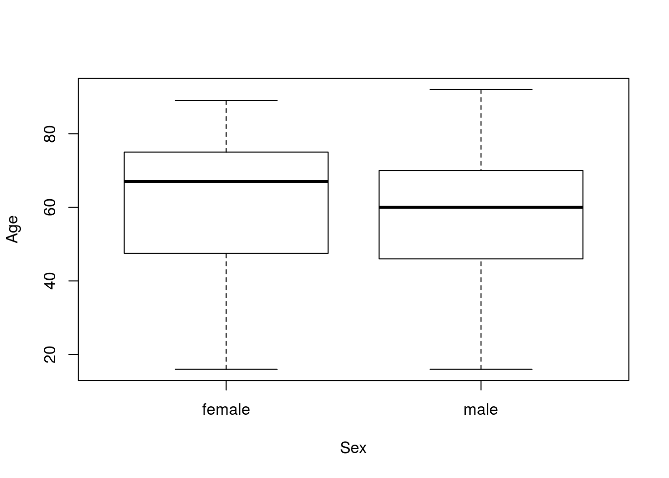
These look a bit diffent, though there seems to be a lot of overlap. Next, let’s save the values to separate variable to make our code a bit easier.
# Save variable (not always necessary)
menAge   <- icu$Age[icu$Sex == "male"]
womenAge <- icu$Age[icu$Sex == "female"]
Then, we can see how different the means are. This is our point estimate of the difference:
ptEst <- mean(womenAge) - mean(menAge)
ptEst
## [1] 3.959677So, women are 3.96 years older than men in this sample. But: is this difference significant? For that, we need to first know how many standard errors our observed data are from the null expecation. For that, we calculate the standard error:
# Calculate SE
ageSE <- sqrt( sd(  menAge) ^ 2 / length(  menAge) +
               sd(womenAge) ^ 2 / length(womenAge) )
ageSE
## [1] 2.965941Now, instead of using this SE with a t-critical value to calculate a margin of error, we instead want to convert our observed data to a t-statistic. That is, just like calculating the z-statistic for the proportion tests, we want to know how different our observed data are from the expected null measured in standard errors, instead of the origninal units.
# Calculate t-stat (z-score)
ageTstat <- ptEst / ageSE
ageTstat
## [1] 1.335049So, our data are about 1.335 SE away from our null expectation. That doesn’t seem like a huge number, but to see how likely we are to get that by chance, we need to use pt(). For that, we need to calculate our degrees of freedom. Recall that we are basing this on our smaller n value (for now).
# Calculate degrees of freedom
ageDF <- min(length(  menAge),
             length(womenAge)) - 1
ageDF
## [1] 75Finally, we use this (and our t-statistic) in pt(), to get our p-value. Since our HA is two-tailed, we need to double it. Note that I am using the negative of the absolute value (which will always be negative), so that I don’t need to think about whether or not to subtract from 1 (it is always the left tail).
# Calculate one-tailed p
pt(-abs(ageTstat), ageDF)
## [1] 0.09294923# Double for two tailed
2 * pt(-abs(ageTstat), ageDF)## [1] 0.1858985So, we expect to see a difference this large, or larger, about 19 times in 100 similar tests. That certainly doesn’t seem very rare or unlikely, so we would fail to reject the null hypothesis of no difference. This does not mean that men and women in the ICU are the same age, only that we do not have enough evidence to say that they are different ages.
27.4.1 Try it out
Are the heart rates (column HeartRate) differnent between patients in for “medical” or “surgery” visits (column Service). Make sure to plot the difference. You should get something like this:
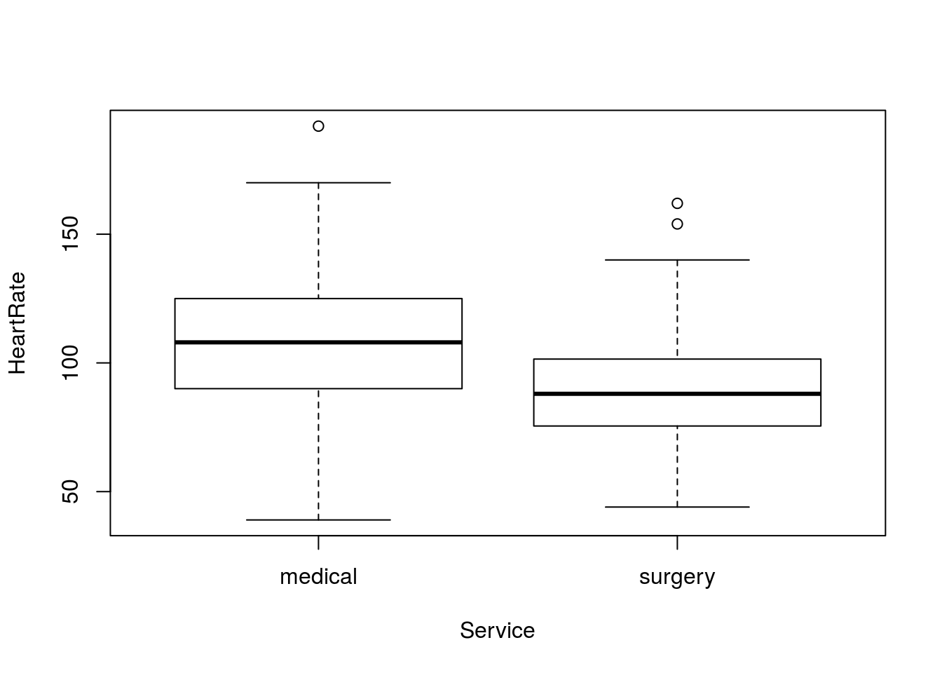
Or this:
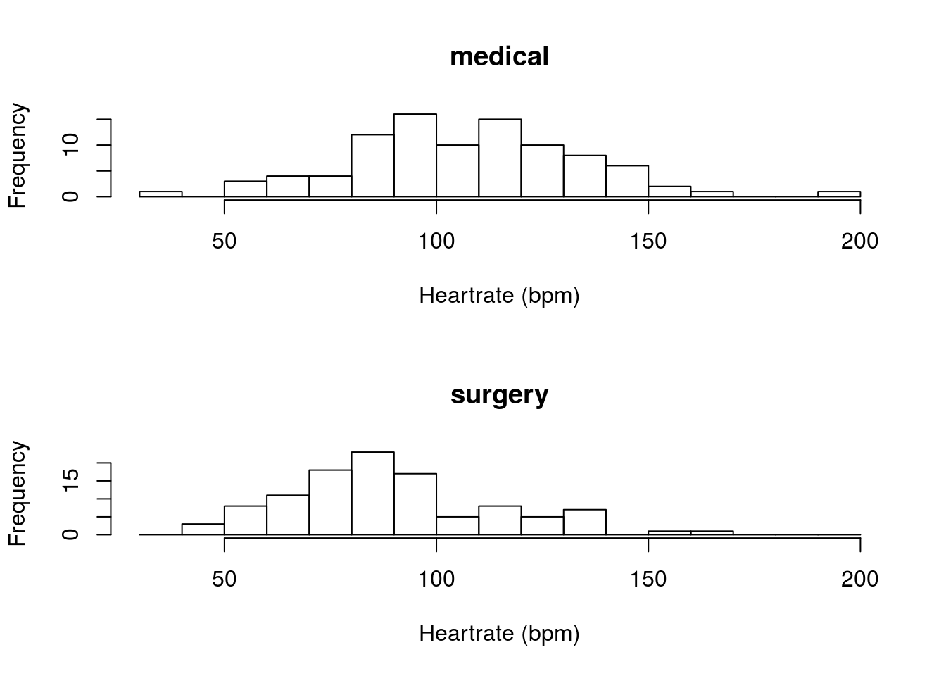
You should get a p-value of 0.00000493. Make sure that you think carefully about what this means.
27.5 An example with given values
We can also apply these methods to supplied numbers, instead of from data. For this, I am largely copying from above, but just replacing the calculations with given values.
Imagine that a very expensive restaraunt wanted to know if the bills paid by credit card were a different mean amount than bills paid by other methods (e.g. cash or check). The mean bill paid by credit card was $200, with a sample sd of $20 from 30 bills; while the mean bill paid by cash was $190, with a sample sd of $30 from 35 bills. Are these means different?
Let’s start by just entering all of the values we were given.
# Set credit info
credMean <- 200
credSD   <-  20
credN    <-  30

# Set cash info
# Can copy above, then use find replace
cashMean <- 190
cashSD   <-  30
cashN    <-  35
Giving us the data:
| mean | sd | n | |
|---|---|---|---|
| credit | 200 | 20 | 30 |
| cash | 190 | 30 | 35 |
From here, we can just progress through the rest of the steps with no problems. We can use those values to calculate our SE. Note here that we have a supplied value for our standard deviations and N, rather than calculating them on the fly with sd() and length() – for some this may help to clarify the steps we took above.
# Calculate SE
diffSE <- sqrt( ( credSD ^ 2 / credN ) +
                ( cashSD ^ 2 / cashN ) )
diffSE
## [1] 6.248809So, the SE we would use for all of our other calculations (e.g., as the denominator for our t-statistic) would be 6.2488.
Next, we need to calculate (and save) our point estimate of the difference, and convert it to a t-statistic Note that you could also do this if all you were given were a difference simply by saving that as your diffMean variable.
# Calculate difference
diffMean <- credMean - cashMean
diffMean
## [1] 10# Calculate t-stat (z-score)
myT <- diffMean / diffSE
myT## [1] 1.600305So, the difference between our means is about 1.6 standard errors. To see how likely we are to get that by chance, we need to use pt(). For that, we need to calculate our degrees of freedom.
# Calculate degrees of freedom
myDF <- min(credN, cashN) - 1
myDF
## [1] 29Finally, we use this (and our t-statistic) in pt(), to get our p-value. Since our HA is two-tailed, we need to double it. Note that I am using the negative of the absolute value (which will always be negative), so that I don’t need to think about whether or not to subtract from 1 (it is always the left tail).
# Calculate one-tailed p
pt(-abs(myT), myDF)
## [1] 0.06018507# Double for two tailed
2 * pt(-abs(myT), myDF)## [1] 0.1203701So, we expect to see a difference this large, or larger, about 12 times in 100 studys. This doesn’t seem very remarkable, so we probably don’t reject the null hypothesis. The two means might be the same, though we can’t say that for sure.
27.5.1 Try it out
Imagine that you sampled the mean temperature of a number of home-brewed cups of coffee and a number of cups bought at Starbucks. Given the data below, test whether or not the mean temperature of the coffee differs between home and Starbucks.
| Starbucks | Home | |
|---|---|---|
| mean | 180 | 175 |
| sd | 2 | 3 |
| n | 8 | 10 |
You should get a p-value of 0.0039.
27.6 Paired differences
Sometimes, we know a little bit more about our data, and we want to use that information. Let’s start by looking at some of the class grades, specifically, I might be interested in knowing if some pair of two quizzes were different difficulties. Here, let’s compare lab quiz 6 (column labQuiz06) against the lecture quiz 3 (column classQuiz03). As always, we start with our hypotheses:
H0: The mean percentage score on lab quiz 6 is equal to the mean percentage score on lecture quiz 3
HA: The mean percentage score on lab quiz 6 is not equal to the mean percentage score on lecture quiz 3
This will require some extra manipulation as the lab quizzes are out of 5 points, and the class quizzes are out of 10 points. To handle this, we will represent each as a percentage score and save them in their own variable.
# Store the variables
labQ <- classGrades$labQuiz06 / 5
lecQ <- classGrades$classQuiz03 / 10
We can then plot those scores:
boxplot(labQ, lecQ,
        names = c("lab","lecture"),
        xlab = "Quiz type",
        ylab = "Percent score")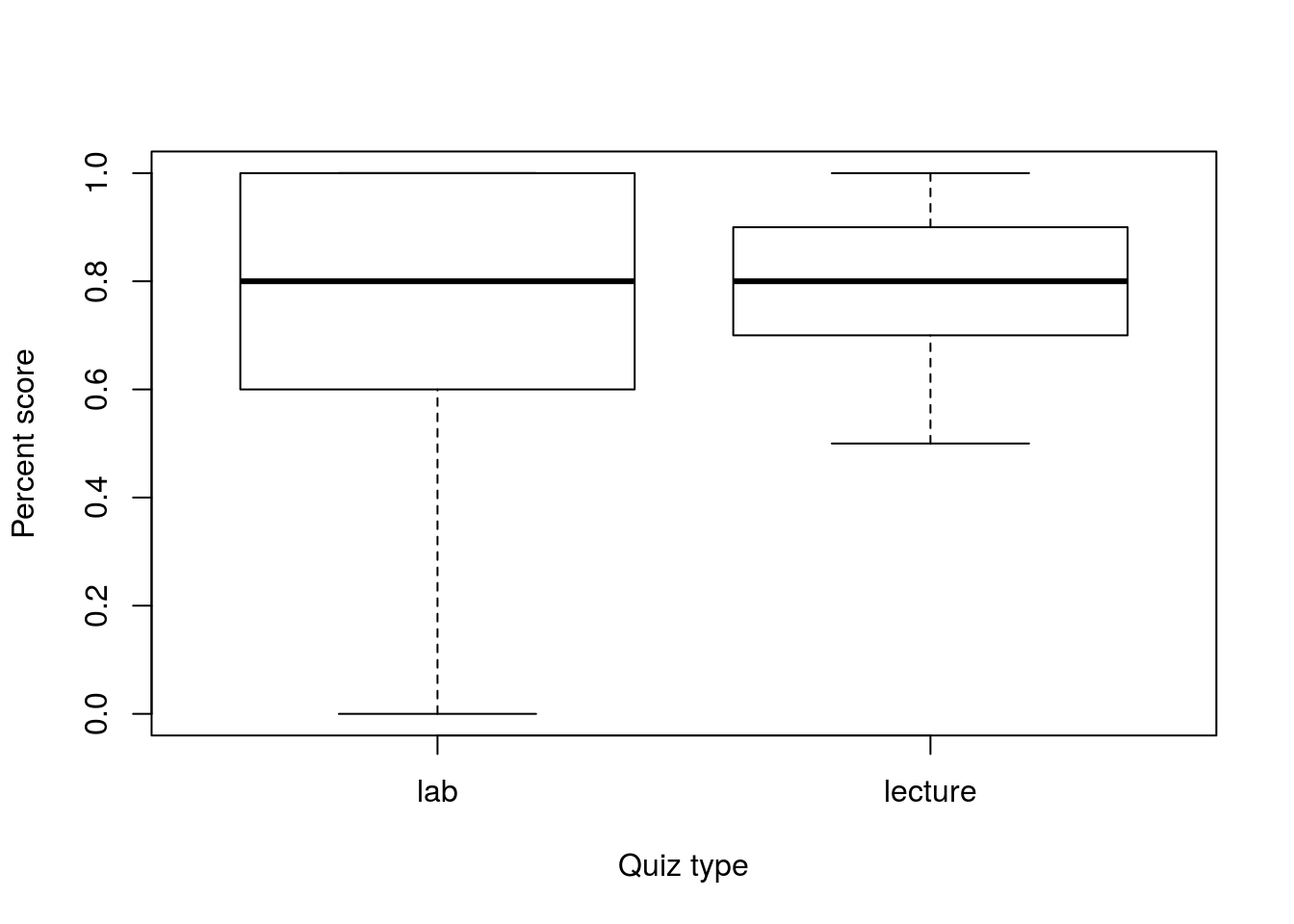
These scores look pretty similar, but not quite identical. So, we can use the above steps (abbreviated explanation here) to calculate a p-value:
# Store the difference
diffMean <- mean(lecQ) - mean(labQ)

# Calculate SE
diffSE <- sqrt( sd(lecQ) ^ 2 / length(lecQ) +
                sd(labQ) ^ 2 / length(labQ) )

# Calculate degrees of freedom
myDF <- min(length(lecQ), length(labQ)) - 1

# Calculate t-statistic
myT <- diffMean / diffSE

# Calculate p-value
myP <- 2*pt(-abs(myT), df = myDF)
myP
## [1] 0.1028443This gives us a p-value of 0.103, and would lead us to not reject the null hypothesis. However – we know a little bit more about these data. Not all students are the same, and we know which student (anonymized here) took each quiz. We can see this if we plot the scores against each other:
plot(labQ ~ lecQ)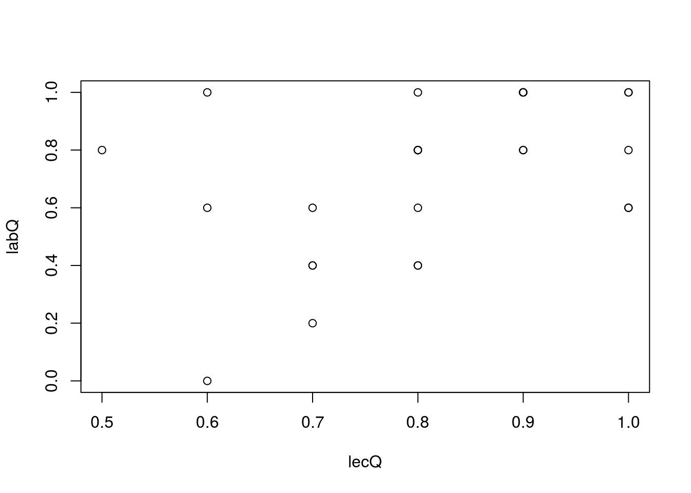
While there is not a particularly strong correlation, we can still see that students that did well on the lecture quiz also did well on the lab quiz. That means that some of the variation in our data, which is getting added to the SE we calculate, is just noise caused by the difference between students. We can handle this by making a slight tweak to our hypotheses:
H0: The mean percentage score for each student is equal on lab quiz 6 and lecture quiz 3
H0: The mean percentage score for each student is not equal on lab quiz 6 and lecture quiz 3
Here, we are asking about the difference in scores for the two quizzes. This is called a “paired” test because we are “pairing” the scores on the two quizzes for each student. So, we can save the difference:
# Save the actual differences
quizDiff <- lecQ - labQ

# Plot it
hist(quizDiff, breaks = 10)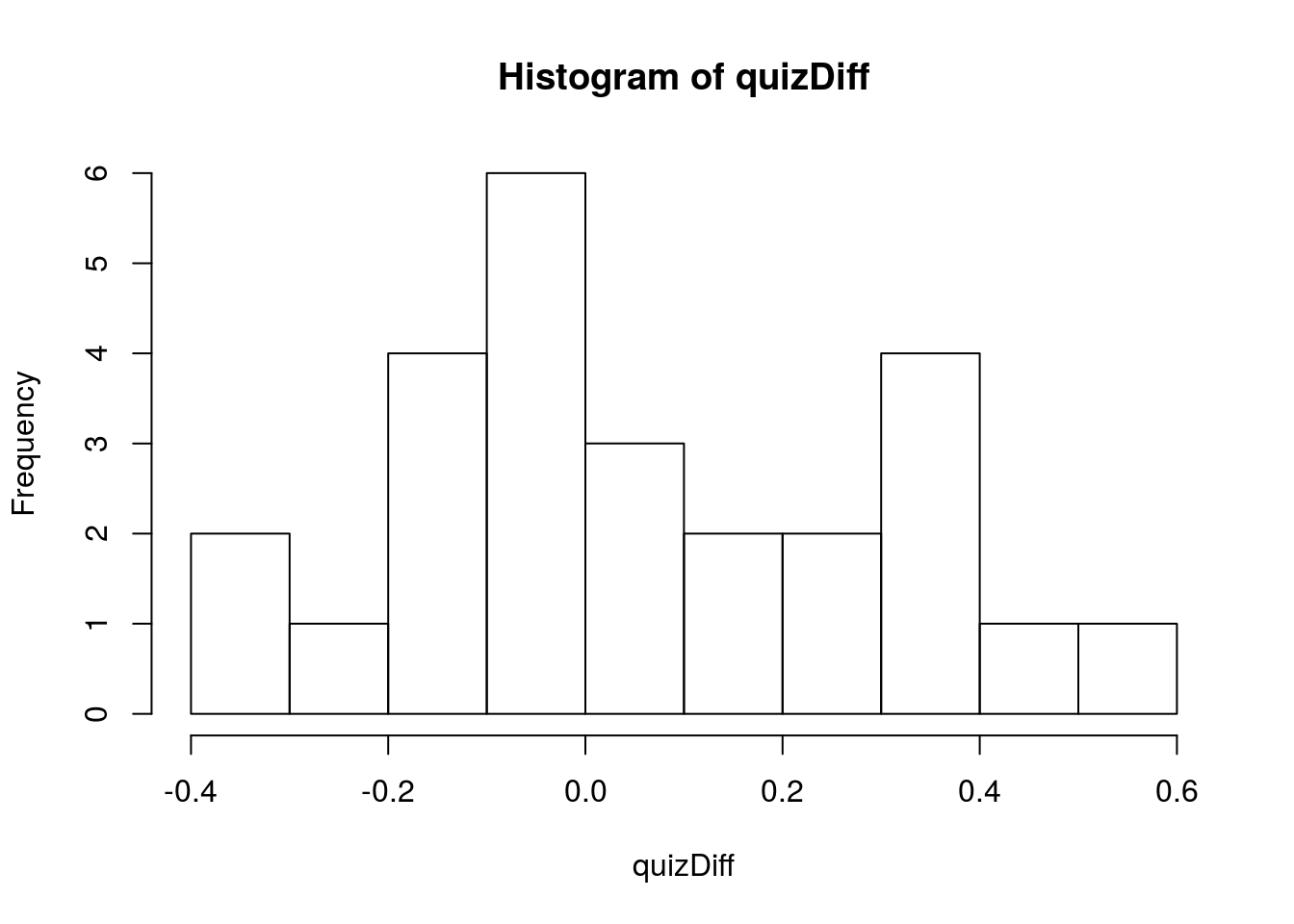
This makes it look like, on average, there is a slight bias towards scores on the lecture quiz being a little higher. The differnce between the two means is the same as the mean of the differences, but now our calculations work a little bit differently. Specifically, we can now treat the variable quizDiff as a single sample and use the tests of a single mean, treating 0 as our H0 because our H0 is the same as saying that the average difference is 0. So, we can apply our one-sample methods, again shown with minimal description:
# Calculate SE
pairSE <- sd(quizDiff) / sqrt(length(quizDiff))

# Store t-statistic
pairT <- mean(quizDiff) / pairSE

# Calculate p-value
pairP <- 2*pt(-abs(pairT),
              df = length(quizDiff)-1 )
pairP
## [1] 0.04599271This now gives us a p-value of 0.046, which is low enough to reject our null hypothesis of no difference (using our common threshold of 0.05). Thus, we were able to use the additional information at our disposal to show that, on average, it appears that lecture quiz 3 was harder than lab quiz 6.
27.6.1 Try it out
Were lab quiz 7 and lecture quiz 6 the same difficulty for each student? Make sure to state your hypotheses and run an appropriate test. Don’t forget that the lab quiz is out of 5 and the lecture (class) quiz is out of 10 (Like I did when I first calculated the value to put here).
You should get a p-value of 0.174.