An introduction to statistics in R
A series of tutorials by Mark Peterson for working in R
Chapter Navigation
- Basics of Data in R
- Plotting and evaluating one categorical variable
- Plotting and evaluating two categorical variables
- Analyzing shape and center of one quantitative variable
- Analyzing the spread of one quantitative variable
- Relationships between quantitative and categorical data
- Relationships between two quantitative variables
- Final Thoughts on linear regression
- A bit off topic - functions, grep, and colors
- Sampling and Loops
- Confidence Intervals
- Bootstrapping
- More on Bootstrapping
- Hypothesis testing and p-values
- Differences in proportions and statistical thresholds
- Hypothesis testing for means
- Final thoughts on hypothesis testing
- Approximating with a distribution model
- Using the normal model in practice
- Approximating for a single proportion
- Null distribution for a single proportion and limitations
- Approximating for a single mean
- CI and hypothesis tests for a single mean
- Approximating a difference in proportions
- Hypothesis test for a difference in proportions
- Difference in means
- Difference in means - Hypothesis testing and paired differences
- Shortcuts
- Testing categorical variables with Chi-sqare
- Testing proportions in groups
- Comparing the means of many groups
- Linear Regression
- Multiple Regression
- Basic Probability
- Random variables
- Conditional Probability
- Bayesian Analysis
CI and hypothesis tests for a single mean
23.1 Load today’s data
- NFLcombineData.csv
- Data on the Height, Weight, and position type of all 4299 players that participated in the NFL combine during the collection period
- icuAdmissions.csv
- Data on patients admitted to the ICU.
# Set working directory
# Note: copy the path from your old script to match your directories
setwd("~/path/to/class/scripts")

# Load data
nflCombine    <- read.csv("../data/NFLcombineData.csv")
icu           <- read.csv("../data/icuAdmissions.csv")
23.2 Confidence intervals
These standard distributions are great if you are generally interested in the t-distribution, but far less useful if we are interested in actual data (which does not generally have mean of 0 and sd of 1). Thus, we will need to convert our data to z-scores to calculate probabilities, and convert the quantiles from the z-distribution to critical values on our scale (this is the purpose of the z* for the normal distribution).
23.2.1 Quantiles to calculate confidence intervals
For now, to calculate confidence intervals, we want to be able to convert calculated quantiles to our scale. This is equivalent to the z-critical (z*) methods for the normal. The process here is essentially:
- Calculate a threshold on the standardized scale
- Multiply by our sd to return to our scale (this is value is the “margin of error”)
- Add and subtract the margin of error from our mean to get the confidence interval
So, if we have a case with 5 degrees of freedom (to continue our trend), and are interested in a 90% CI, we can calculate our threshold t value (t-critical), often referred to as t*, with relative ease
# Calculate t thresholds
qt(c(0.05,0.95),df = 5)
## [1] -2.015048 2.015048Note here that, because the values are just the negatives of each other, this is often written as “mean ± error”, which is generally read as “the mean plus or minus the margin of error”, and thus only need to type/paste the value once.
However, to get it back to the scale of the data, we first need to multiply by the sd we are using (again, almost always calculated from the data). As an illustrative example, we can assume that we have data with a standard deviation of 5. So, our actual margin of error is:
# Calculate margin of error on "original" scale
qt(c(0.05,0.95),df = 5) * 5
## [1] -10.07524 10.07524So, we might interpret this as having 90% confidence that the true population mean will fall within 10.075 units of whatever our mean is. So, to calculate our actual confidence interval, we need to add/subtract these from our mean. Luckily, they already have the right signs for this. If we had data with a mean of 30, we would then calculate our 90% CI as:
# Calculate the CI
30 + qt(c(0.05,0.95),df = 5) * 5
## [1] 19.92476 40.0752423.3 An actual CI example
Alright, let’s put all of that into practice. Let’s return to our example from the last chapter and calculate a 95% confidence interval for the the heart rate of coma patients. We will then compare that to our bootstrap calculation. First, set up the data as we did in the last chapter.
# Save the data for easy access:
comaSyst <- icu$Systolic[icu$Consciousness == "coma"]

# Plot the values
hist(comaSyst)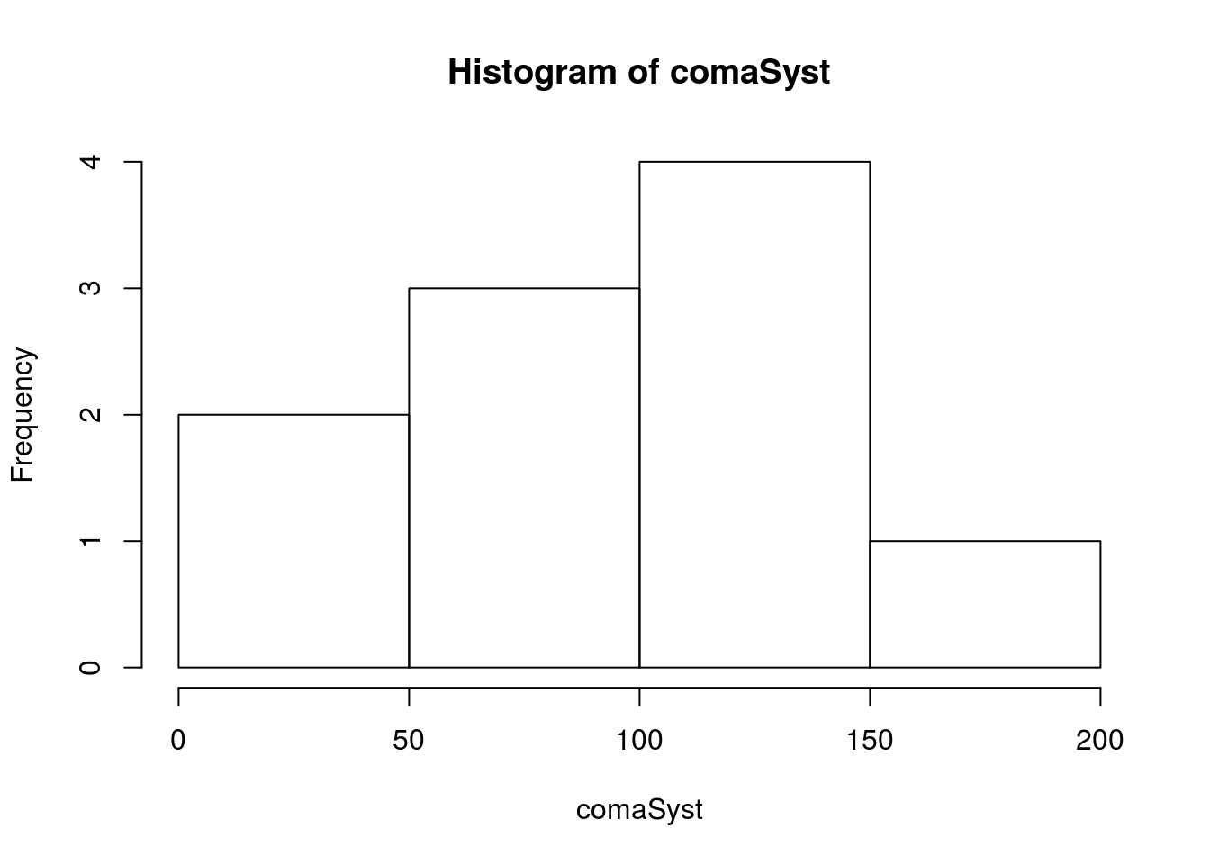
Next, let’s calculate the values we will need:
- the sample size, to scale our t-distribution and sd,
- the mean, for our point estimate and center, and
- the standard error, for our CI
We will then use the sample size to calculate degrees of freedom for the critical/threshold t-values to set our cutoffs, and re-scale them to calculate our CI.
Here, I am going to save all of the values and display them at once, just for the sake of convenience, but you could look at them as you go instead, if you would rather.
# Calculate above values
myN    <- length(comaSyst)
myDF   <- myN - 1
myMean <-   mean(comaSyst)
mySE <- sd(comaSyst) / sqrt(myN)| myN | myDF | myMean | mySE | |
|---|---|---|---|---|
| value | 10 | 9 | 99.4 | 15.4806 |
Now, we can calculate our critical t values:
# Calculate t* for a 95% CI
myTcut <- qt(c(0.025,0.975),df = myDF)
myTcut
## [1] -2.262157 2.262157We then scale by our standard error to get the margin of error:
# Scale to get margin of error
myTcut[2] * mySE
## [1] 35.01954This tells us that we are 95% confident that the true mean blood pressure of coma patients is within 35.02 units (mmHg) of the mean of our sample. To finish it off, we can calculate the actual CI as:
# Calculate the 95% CI
myMean + myTcut * mySE
## [1] 64.38046 134.41954Telling us that we are 95% confident that the true mean blood pressure of coma patients lies between 64.38 and 134.42 with a point estimate of 99.4.
Let’s compare this to the bootstrap calculated values.
# Initialize
bootMean <- numeric()

# Loop
for(i in 1:12345){
  bootMean[i] <- mean(sample(comaSyst,replace = TRUE))
}

# Visualize
hist(bootMean)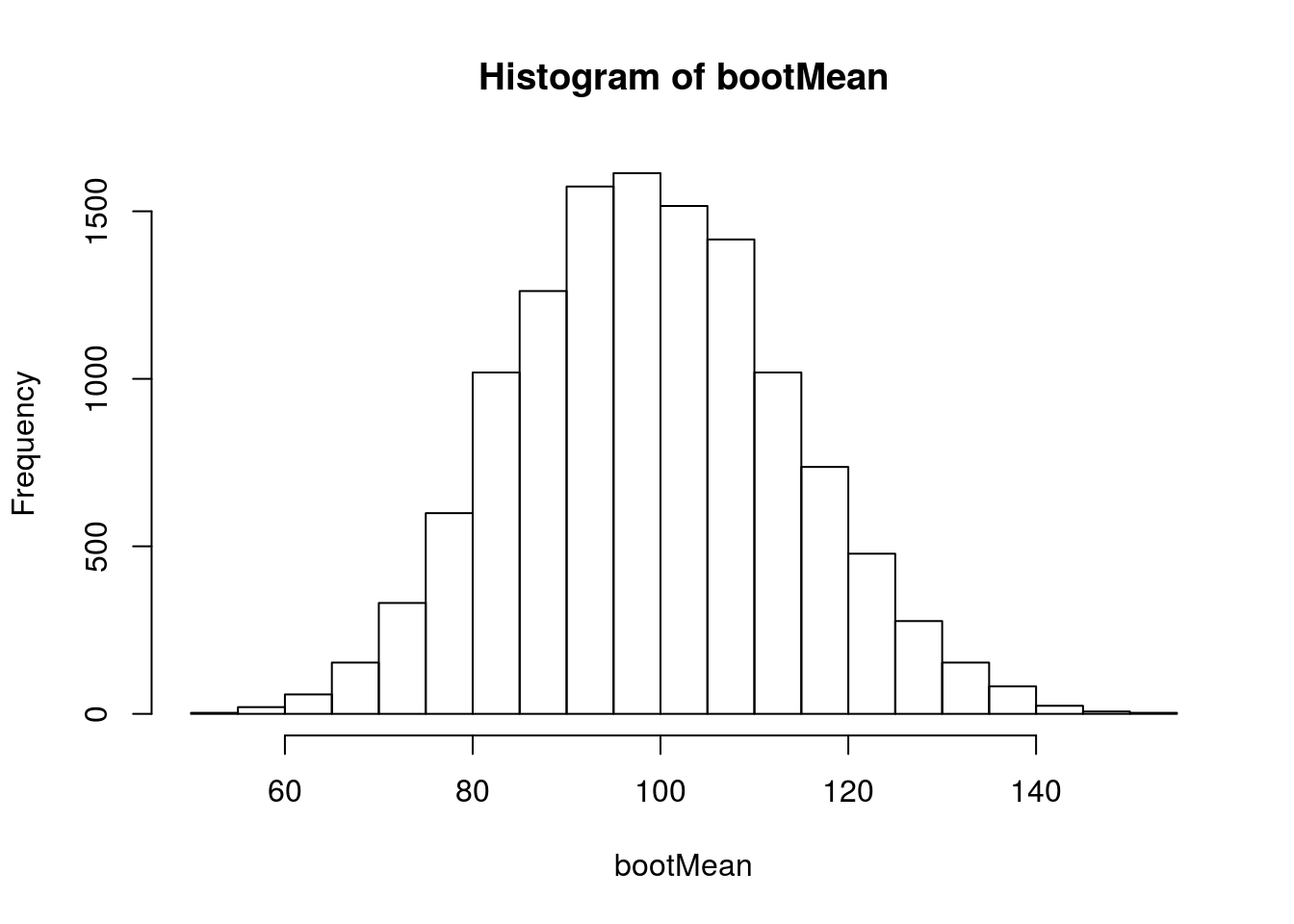
And calculate a 95% CI
# Calculate 95% CI from bootstrap
quantile(bootMean,c(0.025,0.975))
## 2.5% 97.5%
## 71.60 129.08Note that the values are quite close, but that the values calculated from the t-distribution appear to be a little more conservative, reflective of the small sample size.
23.3.1 Try it out
Calculate a 99% confidence interval for the heart rate of patients that had a Fracture (column Fracture has “yes”).
You should find that we are 99% confident that the true mean heart rate of patients with fractures lies between 73.07 and 112.13 with a point estimate of 92.6.
23.4 P-values
Working with p-values on the t-distribution requires a similar conversion to that used for confidence intervals, but in the opposite direction. Calculating probabilities from non-scaled data is as simple as converting your data point to a z-score. Recall that the formula for finding the z-scores for a vector x is just:
( x - mean(x) ) / sd(x)Replacing the x at the begining with the value we are interested in will return a single z-score. Note here, that we could just type in a mean and sd, if we knew them – which is exactly the case when we are testing a null hypothesis. So, if we are interested in finding the probability of getting a value of 6 or less in a t-distribution with mean of 7, sd of 2, and 5 degrees of freedom, we can do the following:
# Calculate the z-score
myZ <- (6 - 7) / 2
myZ
## [1] -0.5# Calculate the probability
pt(myZ, df = 5)## [1] 0.3191494Tells us that about 32% of values in that distribution will be 6 or lower. This would be our (one-tailed) p-value if we were testing the null hypothesis that the mean value was actually 7.
23.4.1 Actual P-value example
In actual use, we would likely be calculating each of those values from our data. The mean is the value of the null hypothesis; the standard error is the sample sd divided by the square root of n; and the degrees of freedom as one less than our sample size.
So, we can return to our coma patient blood pressure, and already have most of the information we need calculated. Let’s say that we are interested in testing the null hypothesis that the mean blood pressure is 120 mmHg with a two tailed alternative.
H0: the mean blood pressure of coma patients equals 120 mmHg
Ha: the mean blood pressure of coma patients does not equal 120 mmHg
We can add a variable for the null hypothesis:
# Set the null hypothesis
myNull <- 120
and just to remind ourselves what all the values are:
| myNull | myN | myDF | myMean | mySE | |
|---|---|---|---|---|---|
| value | 120 | 10 | 9 | 99.4 | 15.4806 |
We see that our observed value is less than our null hypothesis, but is it significantly different? We want to know how likely it would be to get this value (99.4 bpm) if the null is true. So, we need to see how different our observed value is from the null as a z-score (that is, how many standard deviations away from the null is our observed data). As above, we can calculate the z-score as the difference divided by the standard error of the distribution (which we already calculated).
# Calculate the z-score of our observed data
myZ <- (myMean - myNull) / mySE
myZ
## [1] -1.330698Now, we can use pt() to determine how likely that value would be if the null is true. Note that I am using the negative of the absolute value to make sure that I am getting the correct tail of the distribution.
# Calculate p-value
pt(myZ, df = myDF)
## [1] 0.108008Because our alternative is two-tailed, we need to double that value:
# Calculate two-tailed p
2 * pt(myZ, df = myDF)
## [1] 0.216016So, about 20% of the time we collected data, we would expect to get a value as extreme as, or more extreme than, our observed data if the null hypothesis is true. This seems quite likely, so we cannot reject the null hypothesis.
We can also visualize this result, similar to what we have been doing with the histograms following the null distribution loops.
# Plot our t-distribution
curve(dt(x, df = myDF),
      from = -3,
      to   =  3)

# Add lines for our observed values
abline(v = c(myZ, - myZ),
       col = "red3",
       lwd = 3, lty = 3)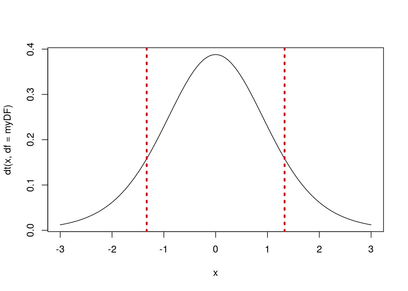
23.4.2 The effect of sample size
This is a good place to remind ourselves that we can never “accept” the null hypothesis. You might be tempted by the above example to conclude that the mean blood pressure of coma patients is 100 mmHg. However, that is not what a failure to reject a null means.
Imagine, for a moment, that the true population value really is 99.4 mmHg. If we were to collect substantially more data, say 100 more patients, we might expect our mean and standard deviation from that sample to still be the same. Note that if the only thing we change is the sample size, we can get a very different answer. The code below is copied from early: only the sample size is changed.
# Calculate needed values
myN    <- 100
myDF   <- myN - 1
myMean <-   mean(comaSyst)
mySE   <-     sd(comaSyst) / sqrt(myN)
myZ <- (myMean - myNull) / mySE| myNull | myN | myDF | myMean | mySE | myZ | |
|---|---|---|---|---|---|---|
| value | 120 | 100 | 99 | 99.4 | 4.895395 | -4.208037 |
Note that changing the sample size dramatically changed the standard error, which in turn made the z-score substantially larger. Now, we calculate the p-value, just as we did above.
# Calculate two-tailed p
2 * pt(myZ, df = myDF)
## [1] 5.670403e-05With this increased sample size, and no other changes, we would now reject the null hypothesis of a mean blood pressure of 100 mmHg. This is an important point to remember as we move forward with these questions. We will explore this idea, referred to as “power” more formally in a coming chapter.
23.4.3 Try it out
Use the data from above on the heart rate of patients with fractures to test the null hypothesis that the mean heart rate of these patients is 110 bpm with a two-tailed test.
You should get a p-value of 0.0189.
23.5 An important reminder
One important point to bear in mind is that the t-distribution assumes a roughly normal distribution after the Central Limit Theorem is applied. So, if you have skewed data and a small sample size, the t-based approximation is not appropriate. Instead, you should probably continue to use the bootstrap approaches, which do not rely on normality.
23.6 For your edification only
The below is for your edification only, and is only included to show you what is possible in R. I will not hold you responsible for any of this, but I thought that it might be of interest.
23.6.1 Scaling curve to display
This is an approach that allows you to plot a t-distribution somewhere other than centered at 0 with sd of 1. It uses the server C credit card tips again.
# Save the data for easy access:
comaSyst <- icu$HeartRate[icu$Consciousness == "coma"]

# Initialize
bootMean <- numeric()

# Loop
for(i in 1:12345){
  bootMean[i] <- mean(sample(comaSyst,replace = TRUE))
}

# Plot histogram
hist(bootMean,freq = FALSE,breaks = 20)

# Add t based only on the initial values (not the boot)
# Note that the effect here is to scale the data to the z-distribution
#  when we pass them to dt, and then divide by the sd when the density
#  is returned to make sure the area under the curve stays the same
mySE <- sd(comaSyst)/sqrt(length(comaSyst))
myMean <- mean(comaSyst)
myDF   <- length(comaSyst) - 1

curve(dt((x-myMean)/mySE, df =  myDF) / mySE,
      add = TRUE,
      col = "blue", lwd = 3)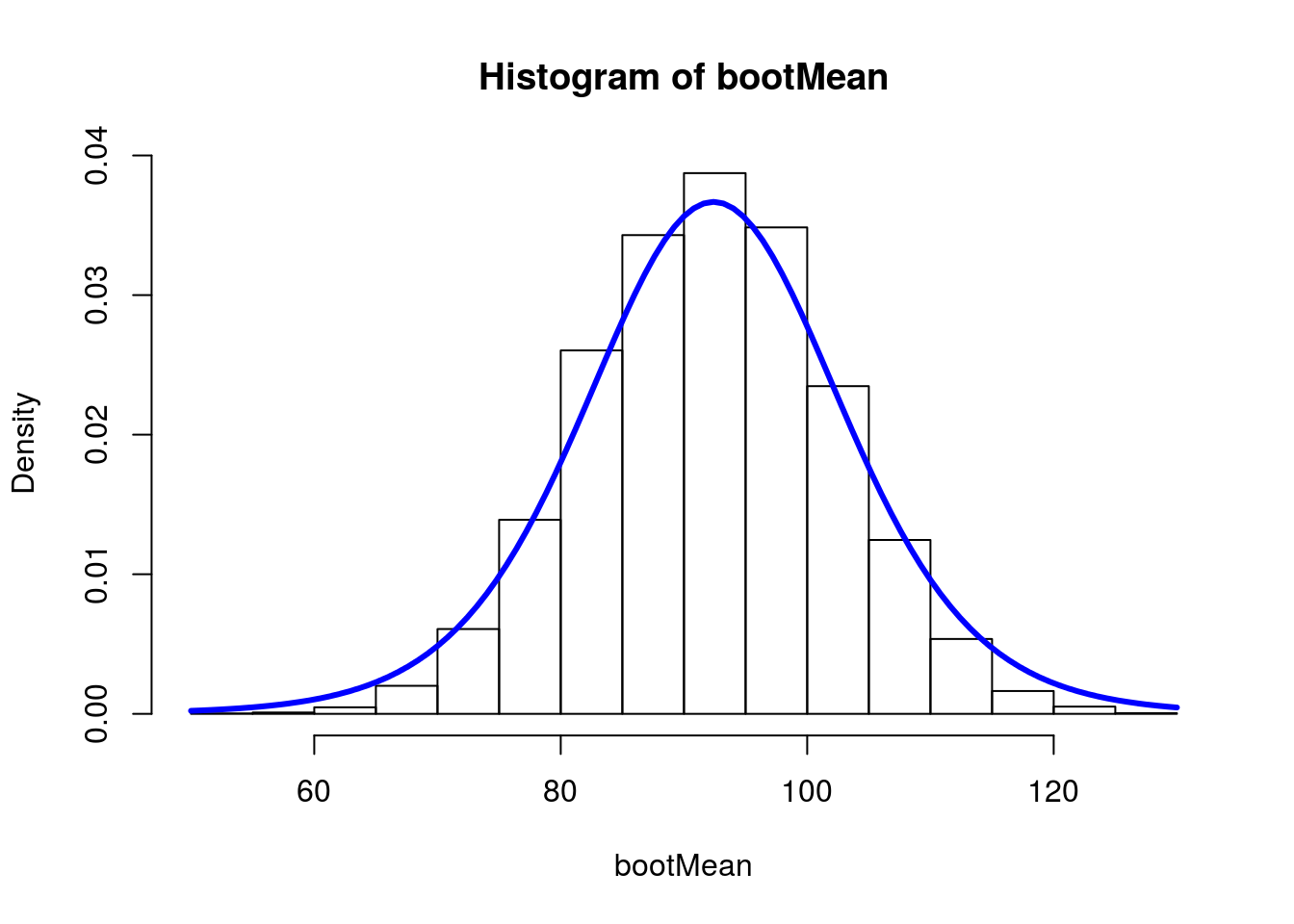
23.6.2 Showing that the CI works
Again, just for your edification. This is to show that the t approximation is a reasonable one.
Here, I will take a bunch of small samples from the NFL population, calculate a CI, and determine if the true population mean is within it or not.
# Save true mean
trueMean <- mean(nflCombine$Weight)

# initialize on variable for t and one for normal
isCloseT <- isCloseNorm <- logical()

# Set sample size
n <- 15

# Set cutoffs, as they will all be the same
tCuts <- qt(c(.025,0.975),df = n -1)
normCuts <- qnorm(c(.025,0.975))

# Loop through lots of samples
for(i in 1:12345){
  # Store sample
  tempSample <- sample(nflCombine$Weight, n)
  tempSD <- (sd(tempSample) / sqrt(n) )

  # Calculate margin of error for each
  margErrT    <- tCuts[2]    * tempSD
  margErrNorm <- normCuts[2] * tempSD

  # Check if sample mean is within margin of error to trueMean
  isCloseT[i]    <- abs(mean(tempSample) - trueMean) < margErrT
  isCloseNorm[i] <- abs(mean(tempSample) - trueMean) < margErrNorm
}

# Look at results
table(isCloseT,isCloseNorm)
## isCloseNorm
## isCloseT FALSE TRUE
## FALSE 647 0
## TRUE 243 11455# What proportion is within CI for the normal?
sum(isCloseNorm) / length(isCloseNorm)## [1] 0.927906# What proportion is within CI for the t?
sum(isCloseT) / length(isCloseT)## [1] 0.9475901Here, we see that our proportion actually within the CI is very close to the confidence level we set (95%) when we use the t-distribution, but is off by a bit more when we use the normal. This will be even more true for smaller sample sizes where the difference in the cutoffs between the normal and T distributions will be larger.