An introduction to statistics in R
A series of tutorials by Mark Peterson for working in R
Chapter Navigation
- Basics of Data in R
- Plotting and evaluating one categorical variable
- Plotting and evaluating two categorical variables
- Analyzing shape and center of one quantitative variable
- Analyzing the spread of one quantitative variable
- Relationships between quantitative and categorical data
- Relationships between two quantitative variables
- Final Thoughts on linear regression
- A bit off topic - functions, grep, and colors
- Sampling and Loops
- Confidence Intervals
- Bootstrapping
- More on Bootstrapping
- Hypothesis testing and p-values
- Differences in proportions and statistical thresholds
- Hypothesis testing for means
- Final thoughts on hypothesis testing
- Approximating with a distribution model
- Using the normal model in practice
- Approximating for a single proportion
- Null distribution for a single proportion and limitations
- Approximating for a single mean
- CI and hypothesis tests for a single mean
- Approximating a difference in proportions
- Hypothesis test for a difference in proportions
- Difference in means
- Difference in means - Hypothesis testing and paired differences
- Shortcuts
- Testing categorical variables with Chi-sqare
- Testing proportions in groups
- Comparing the means of many groups
- Linear Regression
- Multiple Regression
- Basic Probability
- Random variables
- Conditional Probability
- Bayesian Analysis
Approximating a difference in proportions
24.1 Load today’s data
Start by loading today’s data. If you need to download the data, you can do so from these links, Save each to your data directory, and you should be set.
- icuAdmissions.csv
- Data on patients admitted to the ICU.
# Set working directory
# Note: copy the path from your old script to match your directories
setwd("~/path/to/class/scripts")

# Load data
icu           <- read.csv("../data/icuAdmissions.csv")
24.2 Overview
Now that we understand the general ideas of the sampling distribution of a proporition (and other statistics), we can create confidence intervals and calculate p-values. But, far more often, we are interested in the difference between two proportions. For example, are men or women more likely to love President Artman’s?
For that, we need to examine differences between two proportions. We have done this before with bootstrapping. However, as we are starting to see, shortcuts have been developed for a lot of these things.
24.3 Tie example
Recall that we have seen a number of questions like this:
President Artman recently started wearing a new tie. You are interested in knowing how students are responding, particularly whether men and women are responding differently. Instead of asking every student on campus, you surveyed a random subset of students (a good, representative sample). In this survey, you asked each student if they “loved” or “hated” the new tie. Your results:
57 men loved it, 41 men hated it;
227 women loved it, 78 women hated it.
Given this information, we can create a bootstrap distribution to find a confidence interval for the difference between the proportion that love the tie among men and women. We will walk through that again here, then take a look at how we can start using the normal approximation shortcuts to ask the same question.
First, we need to enter our data, including saving the observed proportions (and seeing their difference).
# Save the responses
maleResponses <- c(rep("love", 57),
                   rep("hate", 41))

femaleResponses <- c(rep("love", 227),
                     rep("hate",  78))

# Save point estimates
propMale <- mean(maleResponses == "love")
propFemale <- mean(femaleResponses == "love")

# View the point estimate of the difference
propFemale - propMale
## [1] 0.1626296This suggests that the point estimate for our difference is that women like the tie by 0.16 percentage points.
For the bootstrap:
# Initialize
diffProp <- numeric()

for(i in 1:10283){
  # Collect boot samples
  tempMale <- sample(maleResponses, replace = TRUE)
  tempFemale <- sample(femaleResponses, replace = TRUE)

  # Calculate each proporition
  tempPropMale <-   mean(tempMale   == "love")
  tempPropFemale <- mean(tempFemale == "love")

  # Store the result
  diffProp[i] <- tempPropFemale - tempPropMale

}

# Visualize
hist(diffProp)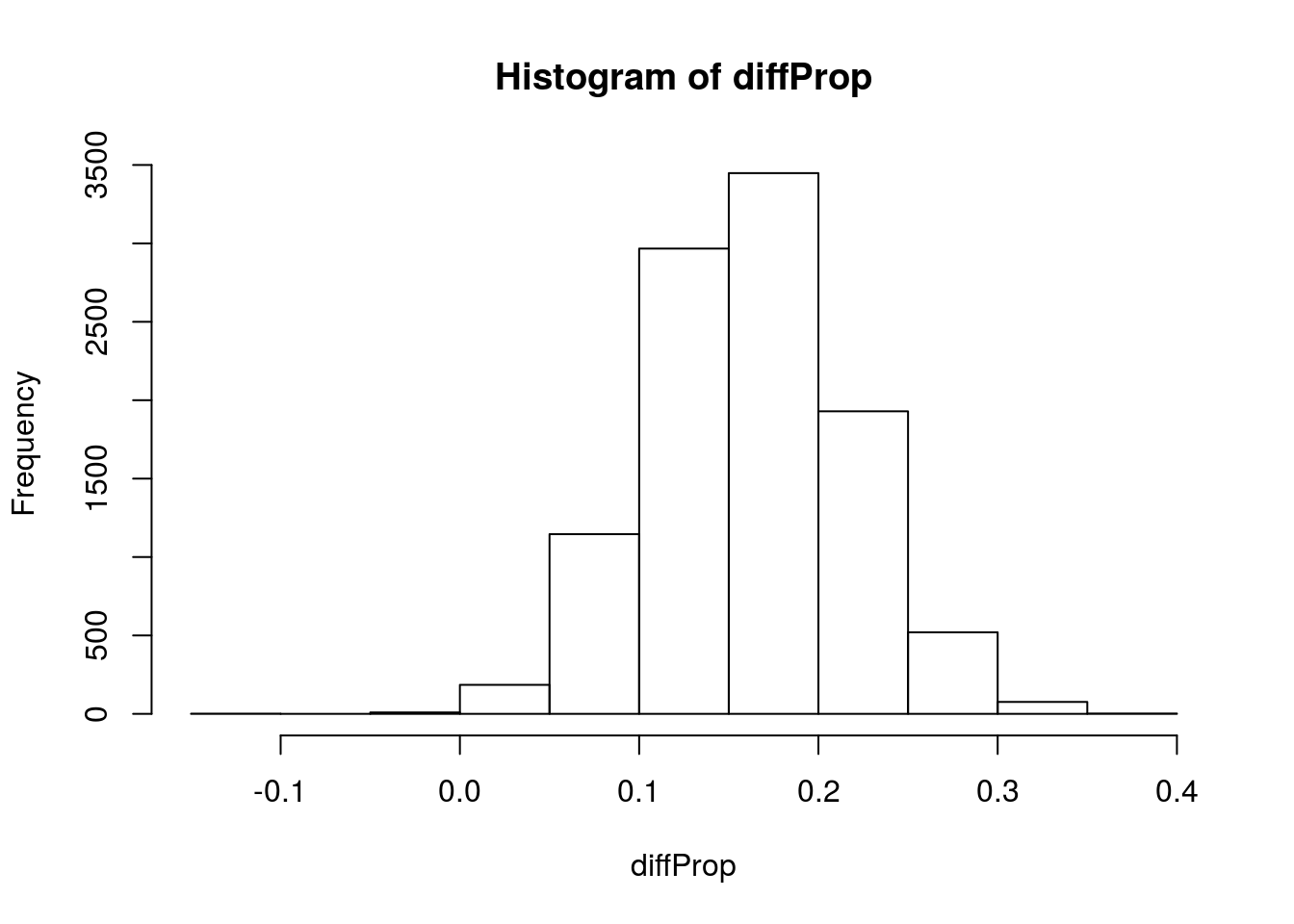
Now, what general shape does that take? Let’s try to model it with the normal.
# Calculate mean
mean(diffProp)
## [1] -0.1622872# Calculate SD
sd(diffProp)## [1] 0.05520493# Add a curve
hist(diffProp,
freq = FALSE,
breaks = 40)
curve( dnorm( x,
mean(diffProp),
sd(diffProp)),
add = TRUE,
col = "red3", lwd = 3)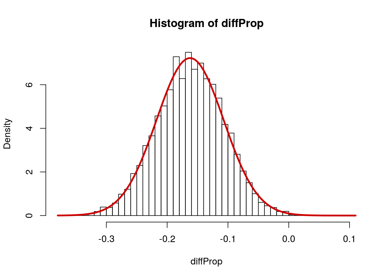
So, the mean is just our point estimate, but what the heck is the standard deviation?
Recall that the standard error for a proportion is \(\sqrt{\frac{p * (1-p)}{n}}\) But how can we get to this from that? It turns out is is a little simpler than we might think, but requires memorizing a new formula:
\[ \sqrt{\frac{p_1 * (1-p_1)}{n_1} + \frac{p_2 * (1-p_2)}{n_2} } \]
Where p1 is the proportion of the first sample, p2 is the proportion of the second sample, and n1 and n2 are the respective sample sizes. For our example, it looks like this:
# Estimate SE
mySE <- sqrt(
  ( propMale * (1 - propMale) / length(maleResponses)) +
  ( propFemale * (1 - propFemale) / length(femaleResponses))
  )

mySE
## [1] 0.05574113Which is very, very close, to the bootstrap result:
# Calculate sd of boot values
sd(diffProp)
## [1] 0.05520493So, now we can model our distribution pretty accurately without having to actually run the bootstrapping.
# Add a curve
hist(diffProp,
     freq = FALSE,
     breaks = 40)
curve( dnorm( x,
              mean = propFemale - propMale,
              sd = mySE),
       add = TRUE,
       col = "darkblue", lwd = 3)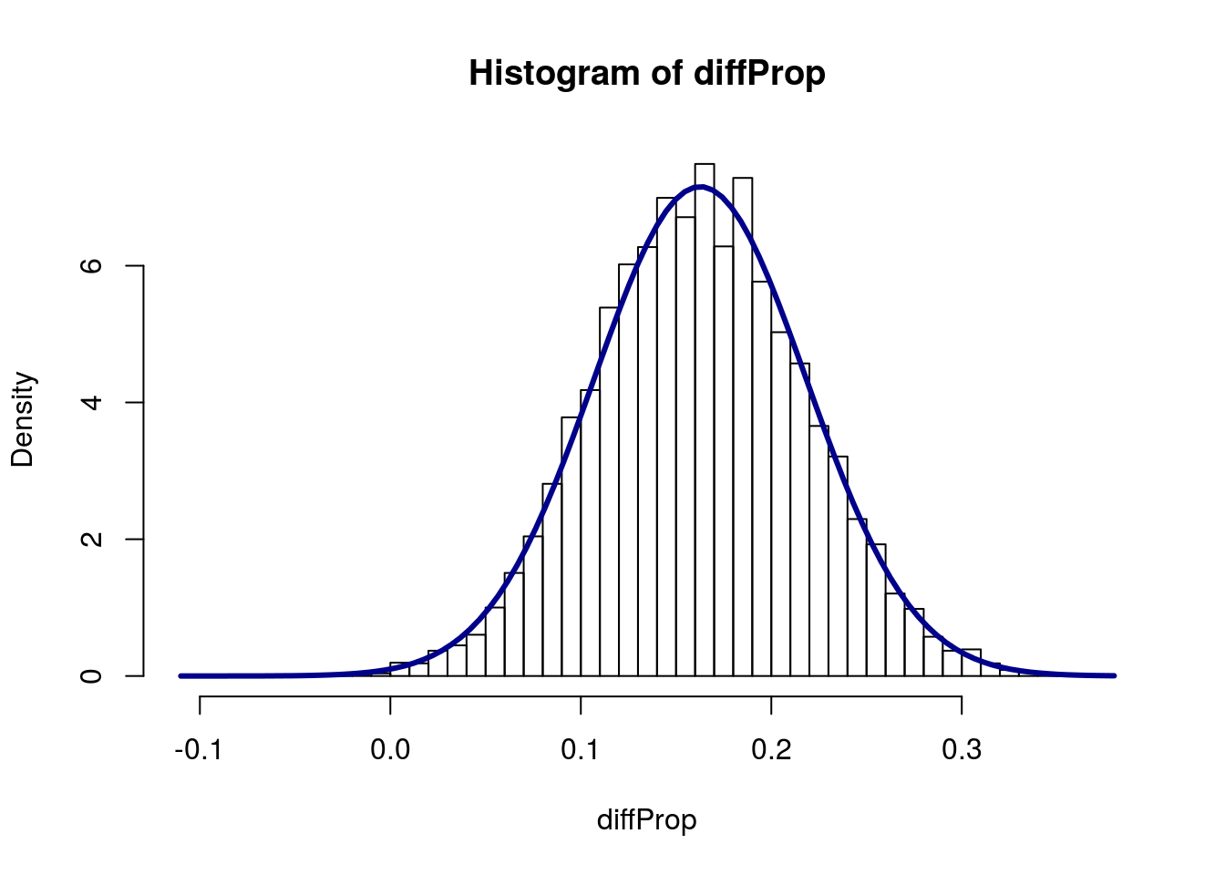
24.4 Using this to calculate a CI
Now that we have these values, we can use them to calculate a confidence interval, just like we have been before. Now, instead of an interval on our estimate of a value, we are asking about an interval on the difference between two values. First, let’s start by visualizing the curve we are talking about.
# Draw the curve
curve( dnorm( x,
              propFemale - propMale,
              mySE),
       from = -0.1 , to = 0.4,
       col = "red3", lwd = 3)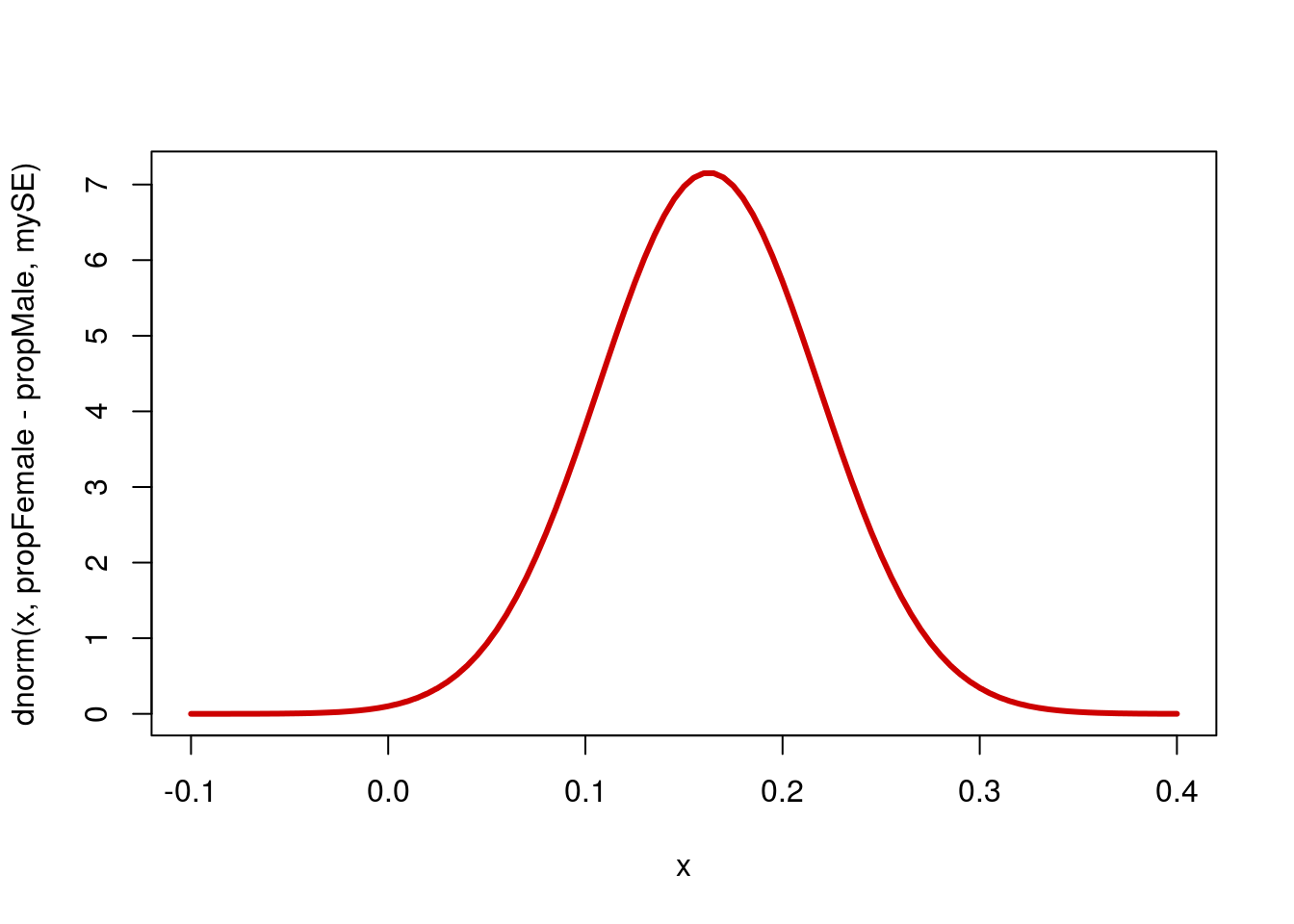
Now, we want to ask where the middle portion of the data lies. Let’s start with a 90% confidence interval.
# Generate critical threshold values
qnorm( c(0.05,0.95) )
## [1] -1.644854 1.644854# Mulitply by SE to get Margin of error
myME <- qnorm( c(0.05,0.95) ) * mySE
myME[2]## [1] 0.091686# Calculate CI by adding/subtracting ME from mean
(propFemale - propMale) + myME## [1] 0.07094364 0.25431564This suggests that we are 90% confident that the true value of the difference lies between 0.0709436 and 0.2543156. Put another way, we are 90% confident that the true difference falls within 0.091686 of our point estimate of 0.1626296. This could also be written as 0.1626296 ± 0.091686. Looking at it on the plot may help.
# Draw the curve
curve( dnorm( x,
              propFemale - propMale,
              mySE),
       from = -0.1 , to = 0.4,
       col = "red3", lwd = 3)

abline(v = (propFemale - propMale) + myME,
       col = "green3", lwd = 3, lty = 2)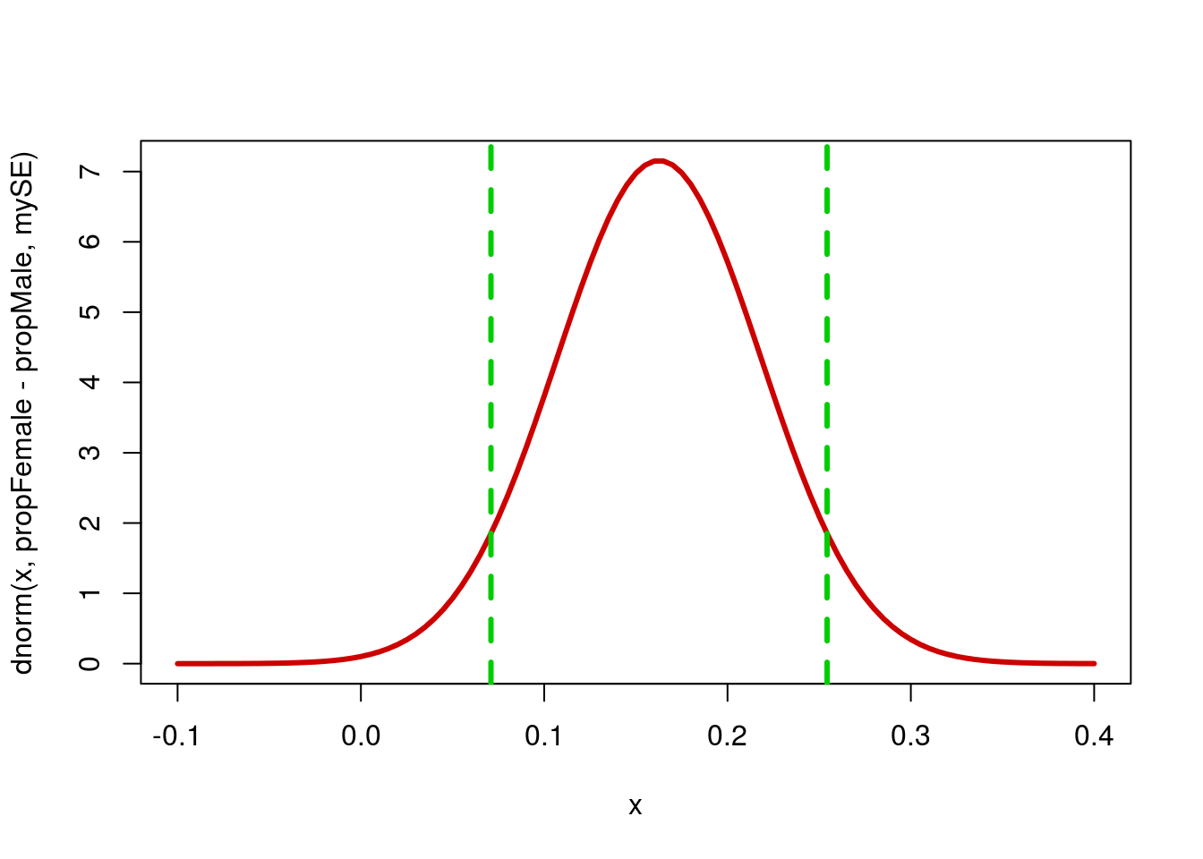
24.4.1 Try it out
Calculate a 95% confidence interval for the difference in proportion of fast zombies that successfully bite someone compared to the proportion of slow zombies that successfully bite someone, given the following data:
16 of 26 tracked fast zombies bit someone before being killed
32 of 44 tracked slow zombies bit someone before being killed
You should find that, given these data, we are 95% confident that the difference in bite rates is between -0.117 and 0.341 (with negative meaning fast zombies have higher proportion successfully biting and positive meaning slow zombies bite successfully more often).
24.5 Working from data
Often, we will be working from data files that are already in the computer. For these, the process is identical, except that we can select the data for our initial vectors, rather than typing it in.
As an example, we can use the icu data to ask about the difference in the proportion of men and women that die in the ICU. First, we select the data for each group:
# Save the data
maleStatus <-   icu$Status[icu$Sex == "male"]
femaleStatus <- icu$Status[icu$Sex == "female"]
From here, we can copy all of the code we used before, changing “Responses” to “Status”.
# Point estimate, copied
propMale <- mean(maleStatus == "died")
propFemale <- mean(femaleStatus == "died")

# Actual point estimate
propMale - propFemale
## [1] -0.01697793Then, we estimate the standard error:
# Estimate SE
mySE <- sqrt(
  ( propMale * (1 - propMale) / length(maleStatus)) +
  ( propFemale * (1 - propFemale) / length(femaleStatus))
  )

mySE
## [1] 0.05869989Finally, use qnorm() to calculate a margin of error here, we can use 99%:
# Mulitply by SE to get Margin of error
myME <- qnorm( c(0.005,0.995) ) * mySE
myME[2]
## [1] 0.1512009and then find the confidence interval:
# Calculate CI by adding/subtracting ME from mean
(propMale - propFemale) + myME
## [1] -0.1681788 0.1342230Thus, we are 99% confident that the true difference in the proportion of patients that die between men and women is between -0.168 and 0.134.
24.5.1 Try it out
Calculate a 90% confidence interval for the difference in the proportion of male and female patients that have been in the ICU before (column Previous == “yes”).
You should discover that we are 90% confident that the true difference in the proportion of patients that have a previous visit between men and women is between -0.144 and 0.033.