25.1 Load today’s data

Start by loading today’s data. If you need to download the data, you can do so from these links, Save each to your data directory, and you should be set.

• icuAdmissions.csv
  • Data on patients admitted to the ICU.

# Set working directory
# Note: copy the path from your old script to match your directories
setwd("~/path/to/class/scripts")

# Load data
icu           <- read.csv("../data/icuAdmissions.csv")

25.2 Overview

We have now introduced sampling distributions for differences in proportions. We have used the confidence interval to estimate the difference between two proportions, but often we simply want to test if two proportions are different. For example, are men or women more likely to vote for Candidate A in an election.

Here, our null hypothesis will always be no difference, noted either as:

H₀: Proportion A = Proportion B

or:

H₀: Proportion A - Proportion B = 0

In either case, we will use the normal model to test how likely it is to have gotten a difference as big (or bigger than) our data by chance if H₀ is true. For most cases, we will use a two-tailed test, though with sufficient a priori justification, you can occasionally use just one. Because the normal (like the t) distribution is symmetrical, we will find the value of one tail and double it.

A one-tailed alternate would then be either:

H_A: Proportion A > Proportion B

or:

H_A: Proportion A - Proportion B > 0

(or < for the opposite direction.) For two tails, we simply use not equal to:

H_A: Proportion A != Proportion B

or:

H_A: Proportion A - Proportion B != 0

After establishing these hypotheses, we will determine how likely the observed data were to have occurred if the null is true.

25.3 An example with the tie data

Recall from the last unit that we were interested in some information about ties:

President Artman recently started wearing a new tie. You are interested in knowing how students are responding, particularly whether men and women are responding differently. Instead of asking every student on campus, you surveyed a random subset of students (a good, representative sample). In this survey, you asked each student if they “loved” or “hated” the new tie. Your results: 57 men loved it, 41 men hated it; 227 women loved it, 78 women hated it.

Now, instead of calculating a confidence interval for the difference, we are going to use it to test the null hypothesis that men and women are equally likely to “love” the tie. That is, we want to know if there is any difference, or if the data are likely to have occurred even if there is not a difference between the sexes. For this, we will use an α of 0.05 to test the following hypothesis (note the two-tailed alternative).

H₀: Proportion of men that love the tie - Proportion of women that love the tie = 0

H_a: Proportion of men that love the tie - Proportion of women that love the tie ≠ 0

Then, copy the input data from the last chapter here.

# Save the responses
maleResponses <- c(rep("love", 57),
                   rep("hate", 41))

femaleResponses <- c(rep("love", 227),
                     rep("hate",  78))

# Save point estimates
propMale <- mean(maleResponses == "love")
propFemale <- mean(femaleResponses == "love")

# View the point estimate of the difference
propFemale - propMale

## [1] 0.1626296

Remember that we will use the formula:

\[ \sqrt{\frac{p_1 * (1-p_1)}{n_1} + \frac{p_2 * (1-p_2)}{n_2} } \]

to estimate the standard error,Where p₁ is the proportion of the first sample, p₂ is the proportion of the second sample, and n₁ and n₂ are the respective sample sizes. For our example, we implemented as this before:

# Estimate SE
mySE <- sqrt(
  ( propMale * (1 - propMale) / length(maleResponses)) +
  ( propFemale * (1 - propFemale) / length(femaleResponses))
            )
mySE

## [1] 0.05574113

However, because our null hypothesis is that the proportions are the same, we don’t want to use separate proportions for each. Instead, we need the proportion of all people that “love” the tie. That is, what proportion of all people love the tie? In practice, this is likely to be a small difference, but it is an important one in many circumstances.

# Pool the responses
pooledResponses <- c(maleResponses, femaleResponses)
# Calculate the pooled proportion
pooledProp <- mean(pooledResponses == "love")

# Estimate SE
mySE <- sqrt(
  ( pooledProp * (1 - pooledProp) / length(maleResponses)) +
  ( pooledProp * (1 - pooledProp) / length(femaleResponses))
            )
mySE

## [1] 0.05296844

So, now, instead of asking for critcal z-values (z*), we are going to calculate our z-score and then calculate how unlikely that is by chance. Recall that the z-score is calculated as:

\[ z = \frac{value - mean}{sd} \]

and for a hypothesis test, we substitute our H₀ for the mean (as it is the center of our predicted sampling distribution) and the standard error for the standard deviation (as it is the measure of spread of our predicted sampling distribution).

\[ z = \frac{data - H_0}{SE} \]

So, for our data, we need to use our point estimate of how different the men and women are to represent our data

# Store the difference
actualDiff <- propMale - propFemale
actualDiff

## [1] -0.1626296

# Calculate Z score
myZ <- (actualDiff - 0) / mySE
myZ

## [1] -3.070312

Then, we figure out how likely it is to get a value as extreme or more extreme using pnorm. Because it is a negative z-value, recall that we need to find the left tail. Thus, we use the output of pnorm directly.

# Calculuate one-tail p-value
pnorm(myZ)

## [1] 0.001069176

If we want to double check that we have the correct tail, let’s graph it.

# Make a standard normal curve
curve(dnorm,
      from = -3.5, to = 3.5,
      lwd = 7, col = "darkblue")

# Add a line where our z-score is
abline( v = myZ,
        col = "green3", lty = 3,lwd = 3)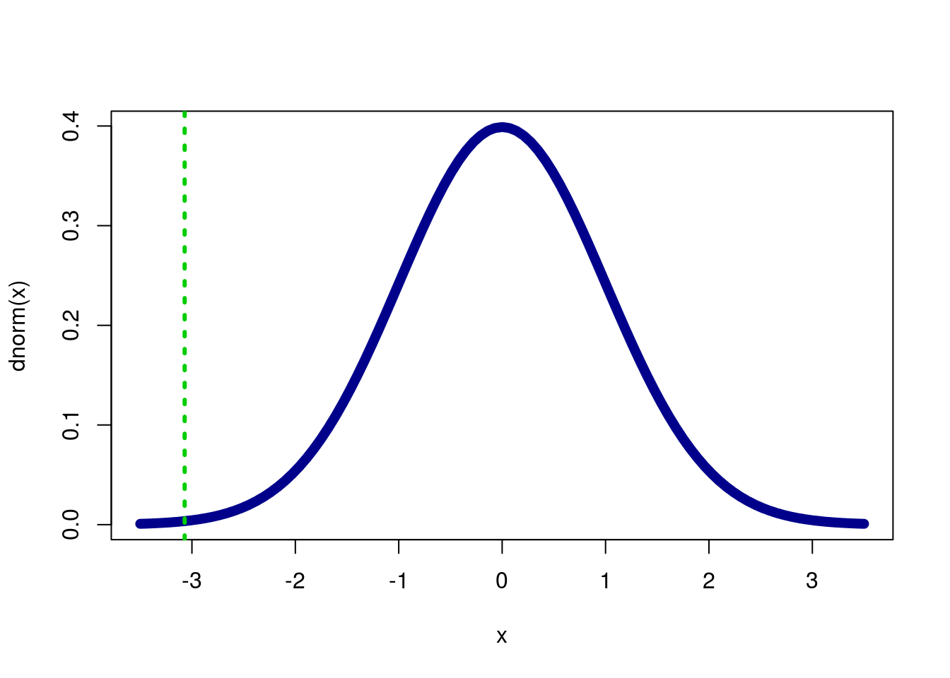

It looks like our p should be very small, and it is.

Now, recall that we want to calculate a two-tailed p-value, so we need to double the one-tailed value. Again, we can see why this is if we plot it.

# Make a standard normal curve
curve(dnorm,
      from = -3.5, to = 3.5,
      lwd = 7, col = "darkblue")

# Add a line where our z-score is
abline( v = c(myZ,-myZ),
        col = c("green3","red3"), lty = 3,lwd = 3)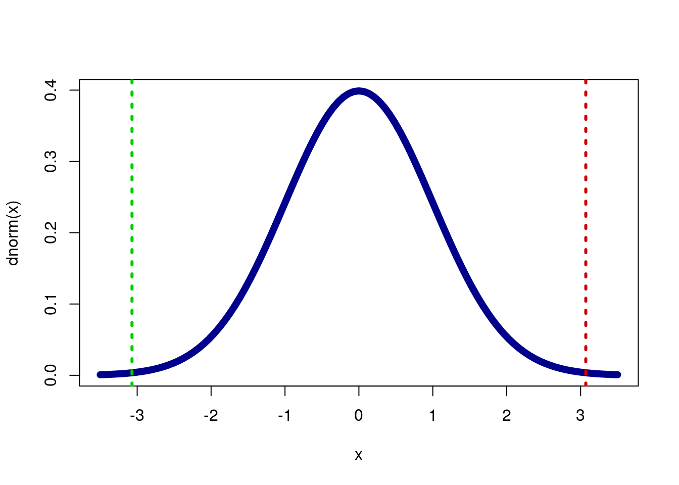

Calculate our two-tailed value now

# calculate two-tailed p-value
pnorm(myZ) * 2

## [1] 0.002138351

Which is quite small, so we reject the null hypothesis that men and women are equally likely to “love” the tie.

25.4 An example with data

As we did when we constructed confidence intervals, let’s see how we can apply this when dealing with data that is already loaded into R.

As an example, we can use the icu data to ask if there is a difference in the proportion of men and women that die in the ICU. First, we state our hypotheses. Our null is going to be the status quo (boring) belief that there is no difference. Because we don’t have any a priori reason to suspect that one sex is more likely to die in the ICU, we will use a two-tailed alternative hypothesis.

H₀: the proportion of men that die in the ICU == the proportion of women that die in the ICU

H_a: the proportion of men that die in the ICU != the proportion of women that die in the ICU

Because we are doing slightly different things with the data this time, we can approach the way we save them differently. Specifically, this time we won’t be using the separated parts often enough to justify first saving them into their own variables. You can do that if you would still like, but here I am showing you how we can use a table() output to do it as well. First, create the table, which shows us the breakdown by sex and status.

# Survival table
survTable <- table(icu$Status, icu$Sex)

addmargins(survTable)

	female	male	Sum
died	16	24	40
lived	60	100	160
Sum	76	124	200

Then, use prop.test() to calculate the proportion of each column that died.

# Save the proportions
props <- prop.table(survTable, 2)
props

##        
##            female      male
##   died  0.2105263 0.1935484
##   lived 0.7894737 0.8064516

Then, we can save the difference between survival rate in the two sexes, which will be used to test our hypothesis.

# Save the data
survDiff <- props["died","female"] - props["died","male"]
survDiff

## [1] 0.01697793

Finally, we need to generate the pooled proportion. This is just the proportion of patients that survived, without any consideration of thier sex. We then use that value to calculate our standard error, which also uses the number of patients of each sex.

# Save pooled proportion
propPool <- mean(icu$Status == "died")

# Calculate the SE
mySE <- sqrt(
  ( propPool * (1 - propPool) / sum(icu$Sex == "male")) +
  ( propPool * (1 - propPool) / sum(icu$Sex == "female"))
  )

Next, we need to determine how many standard errors our data are away from the null hypothesis. (This is the same as calculating a z score, like above.)

# Calculate z
survZ <- (survDiff - 0) / mySE
survZ

##    female 
## 0.2913583

So, we are 0.29 standard errors away from the null hypothesis. We can use pnorm to calculate how likely that is. Remember that we will need to double the size of the tail, as we are running a two tailed test.

Because it is a postive z-value, recall that we need to find the right tail. Thus, we use 1 - the output of pnorm().

# Calculuate one-tail p-value
1 - pnorm(survZ)

##    female 
## 0.3853887

If we want to double check that we have the correct tail, let’s graph it.

# Make a standard normal curve
curve(dnorm,
      from = -3, to = 3,
      lwd = 7, col = "darkblue")

# Add a line where our z-score is
abline( v = survZ,
        col = "green3", lty = 3,lwd = 3)

It looks like our p should be relatively large, but still less than half, and it is. Now, we double it to get our two-tail value

# Find two tailed p
2 * (1 - pnorm(survZ))

##    female 
## 0.7707773

Again, we can see why this is if we plot it.

# Make a standard normal curve
curve(dnorm,
      from = -3, to = 3,
      lwd = 7, col = "darkblue")

# Add a line where our z-score is
abline( v = c(survZ,-survZ),
        col = c("green3","red3"), lty = 3,lwd = 3)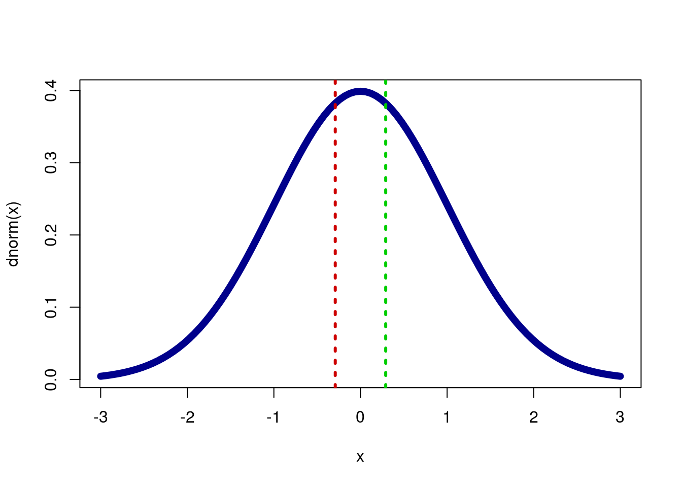

So, with a p-value of 0.7707773 we would fail to reject the null hypothesis that there is no difference in the survival rate in the ICU between men and women. This does not mean that the true proportions are the same, only that we cannot currently say that they are not the same.