An introduction to statistics in R
A series of tutorials by Mark Peterson for working in R
Chapter Navigation
- Basics of Data in R
- Plotting and evaluating one categorical variable
- Plotting and evaluating two categorical variables
- Analyzing shape and center of one quantitative variable
- Analyzing the spread of one quantitative variable
- Relationships between quantitative and categorical data
- Relationships between two quantitative variables
- Final Thoughts on linear regression
- A bit off topic - functions, grep, and colors
- Sampling and Loops
- Confidence Intervals
- Bootstrapping
- More on Bootstrapping
- Hypothesis testing and p-values
- Differences in proportions and statistical thresholds
- Hypothesis testing for means
- Final thoughts on hypothesis testing
- Approximating with a distribution model
- Using the normal model in practice
- Approximating for a single proportion
- Null distribution for a single proportion and limitations
- Approximating for a single mean
- CI and hypothesis tests for a single mean
- Approximating a difference in proportions
- Hypothesis test for a difference in proportions
- Difference in means
- Difference in means - Hypothesis testing and paired differences
- Shortcuts
- Testing categorical variables with Chi-sqare
- Testing proportions in groups
- Comparing the means of many groups
- Linear Regression
- Multiple Regression
- Basic Probability
- Random variables
- Conditional Probability
- Bayesian Analysis
Conditional Probability
36.1 Load today’s data
No data to load for today’s tutorial. Instead, we will be using R’s built in randomization functions to generate data as we go.
36.2 Background
In the previous chapter, we addresed ways of determining the probability of two events occurring. When we wanted to see the probability of two independent events occurring, we simply multiplied their probabilities together. However, often, we will find that our two events are not indpendent. When one thing occurs, the probability of the second may be related.
In the last chapter, we used the example of traffic lights, and explicitly said we need to consider hitting two lights as independent events. However, our own experience likely tells us that this isn’t the case. Lights are timed in such a way that hitting one light green means that we are more likely to hit the next one green as well.
But how can we deal with such events? In this chapter we will explore the concept of conditional probability. This is the idea that the probability of an event depends on what happened in a different event.
36.3 An example
As an example, let’s build an example similar to the one we worked with in the last chapter. Just like with the beads and dice, we will draw a bead then roll a die. The difference this time is that, instead of always rolling a six-sided die, we will roll a different die based on the color of our bead. Specifically, we will roll the die that matches the color of the sampled bead:
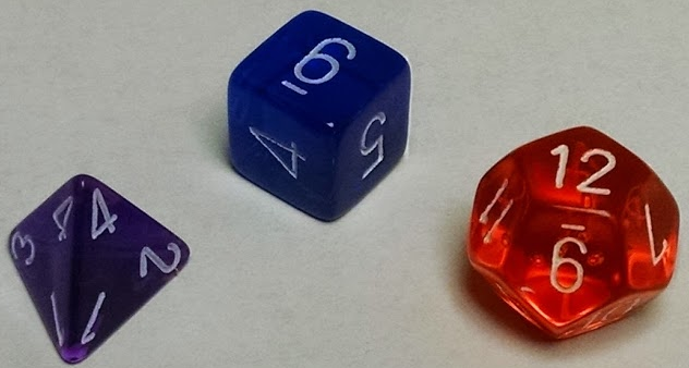
For this example, we will roll:
- a purple four-sided die if we draw a purple bead
- a blue six-sided die if we draw a blue bead, or
- an orange twelve-sided die if we draw an orange bead
For our bead sampling, we will place 15 purple, 20 blue, and 5 orange beads in a cup. We can save these probabilities in R much like we did in the last chapter:
# Save bead colors
beadColor <- c("purple","blue","orange")

# Save probabilities
prob <- c(15, 20, 5)
prob <- prob / sum(prob)
names(prob) <- beadColor
prob
## purple blue orange
## 0.375 0.500 0.125So, this gives us our proability of drawing each bead color.
36.4 Simple example
Given these values, what is the probability of rolling a 12? Only one of our dice can produce a 12, so we know that the probability or rolling a 12 is the same as the probality of drawing an orange bead and rolling a 12. If these were independent, we could use the multiplaction rules from the last chapter. It could look like this:
p(orange & 12) = p(orange) * p(12)
However, you might (rather quickly) notice that we don’t have a single probability of rolling a 12 (p(12)). If we did, we wouldn’t need to care about the color of the bead. Instead, what we need is the probability of rolling a 12 given that we drew an orange bead. this is written as p(A|B), which means “the probability of event A given event B” or, said another way for our example: “If I know that am rolling the orange die, what is the probability that I roll a 12.” In our notation:
p(orange & 12) = p(orange) * p(12|orange)
Because we know that the orange die is a fair 12-sided die, we know that the probability of rolling a 12 is 1/12. So, in R, we can calculate this probability as
# Probability of getting a 12
prob["orange"] * 1/12
## orange
## 0.01041667This shows us that we will roll a 12 about 1.04% of the time that we play this game.
36.4.1 Try it out
Imagine that you know the probability of hitting various lights is:
| trafficLights | probLight |
|---|---|
| red | 0.3 |
| yellow | 0.1 |
| green | 0.6 |
and that the only way you will be early to your destination is if you hit the light at green, and that even then you only have a 40% chance of being early. What is the probability that you will be early?
You should get 0.24.
36.5 Some addition
The above situations asked about a specific outcome: an orange and a 12 or a blue and a 6. What if, instead, we just want to see the probability of getting a 6 with any color bead? We can still ignore the purple, four-sided die, but now it is possible that either the six-sided, blue or the twelve-sided orange die could yield a 6.
In this case, however, it is not possible to draw both a blue and an orange bead. This means that the two probabilities are disjoint and we can apply our simple addition rules from the last chapter. this gives us:
p(6) = p(6 & blue) + p(6 & orange)
Now, for each, we know that the probability of getting that color and number is the probability of getting the color times the conditional probability of getting a six given that we drew the color. Put together, this yields:
p(6) = p(blue) * p(6|blue) + p(orange) * p(6|orange)
Because we are treating them as fair dice, with six and twelve faces respectively, we call the probabilities of getting a 6 1/6 and 1/12 respectively. So, we can calculate the probability as:
prob["blue"] * 1/6 + prob["orange"] * 1/12## blue
## 0.09375So, nearly 10% of the time we play this game, we will get a six.
36.5.1 Try it out
Imagine that you know the probability of hitting various lights is:
| trafficLights | probLight |
|---|---|
| red | 0.3 |
| yellow | 0.1 |
| green | 0.6 |
and that your probability of being on time to your destination is 75% if you hit the light at green, and only 60% if you do not. What is the probability that you will be on time?
You should get 0.69.
36.6 Visualizing conditional probability
One of the trickiest parts about conditional probability can often be developing a visual representation of it. Generally speaking, these are tools that are most useful to sketch out by hand on scratch paper, rather than things to present. R has tools to create them; however, by their very nature, they are tricky to code. If you are interested, I will share the code to make the below plots (the are made with the package diagram), but working with these fall far beyond the scope of this course[*] These were about 50 lines of code each, and that is with judicious use of loops. Each piece of the plot needs to be specified explicitly in this package. If you really want to take the time to make these (e.g., if you need them for a class or work project/presentation), you would probably be better off looking at the TikZ package for LaTeX. .
The most common diagram for conditional probability is called a tree diagram. At each event, the diagram branches to each possible outcome. Then, from each of those events, the possible outcomes of the next event are listed. The conditional probabilities of each are then written along the branches to show the likelihood of each series of events.
As a simple example, let’s imagine a new scenario:
- Suppose there is a 25% chance of rain every day.
- If it rains, there is a 20% chance that you will be late.
- If it does not rain, then there is a 10% chance that you will be late.
From this, we have enough information to figure out the probabilities of every possible outcome (rain vs. no-rain and late vs. on-time). However, it can often be helpful to draw a picture. In this case, we start by showing the probability of rain. Then, for each scenario, show the probability of being late or on-time.
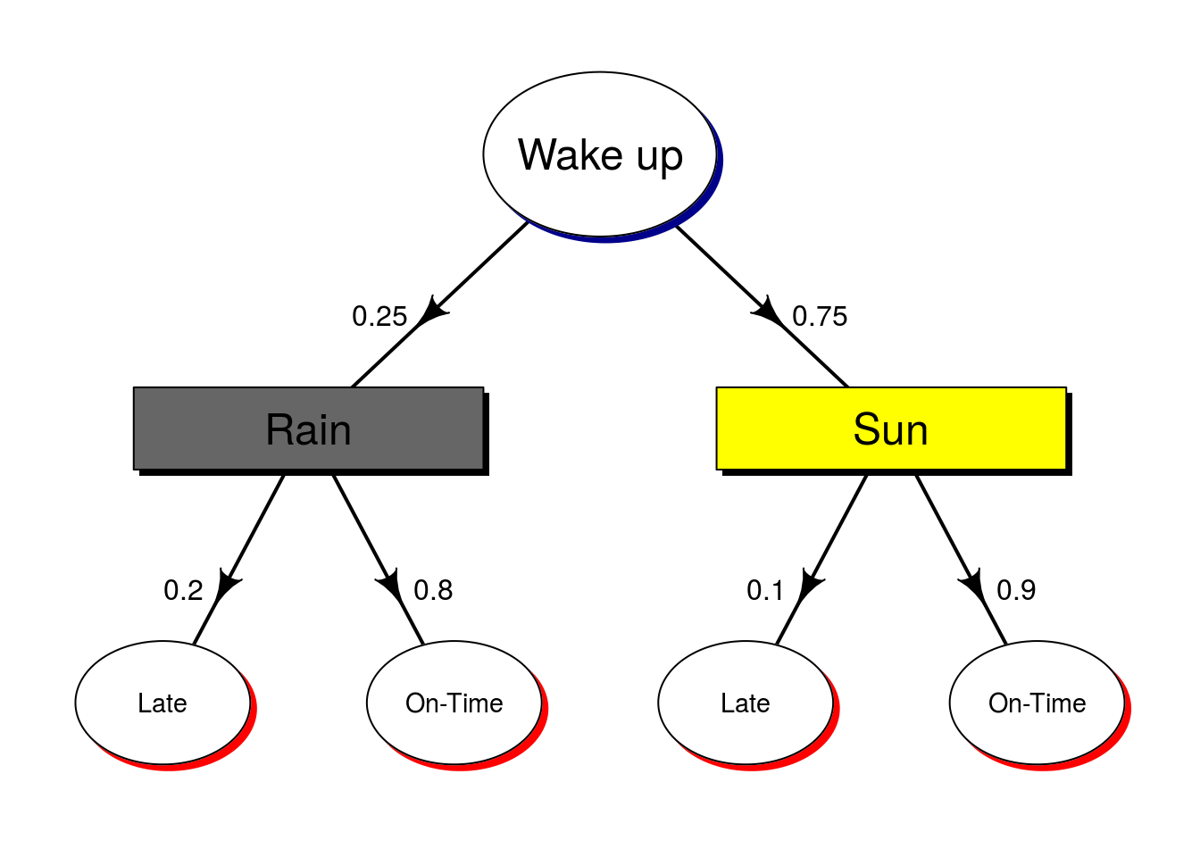
As you can see, this quickly shows us all of the conditional probabilities, which (especially for more complicated scenarios) makes it a lot easier to figure out what things to combine. So, in our case, if we want to know the probability of being late, we can see that we need to combine the probability of being late when it is raining and when it is sunny. In formal notation, that is:
p(Late) = p(Late & Rain) + p(Late & Sun)
Which we can re-write as:
p(Late) = p(Rain) * p(Late | Rain) + p(Late) * p(Late | Sun)
Now, we notice that those are just the numbers along the two sets of arrows leading to the “Late” bubbles. So, a simple heuristic to figure out the probability of an event from a tree diagram is to multiply the probabilities along the path to the final outcome. Here, we use:
p(Late) = 0.25 * 0.2 + 0.75 * 0.1
to get 0.125. So, given these probabilities, you would be Late 12.5% of the time.
36.7 Tree for the dice example
For more complicated scenarios, tree diagrams be can a great way to quickly visualize possible outcomes. When there get to be a lot of arrows, I tend to cluster and label arrows that share the same probabilities. So, because each of our dice is fair, we can just label the group, rather than every single arrow.
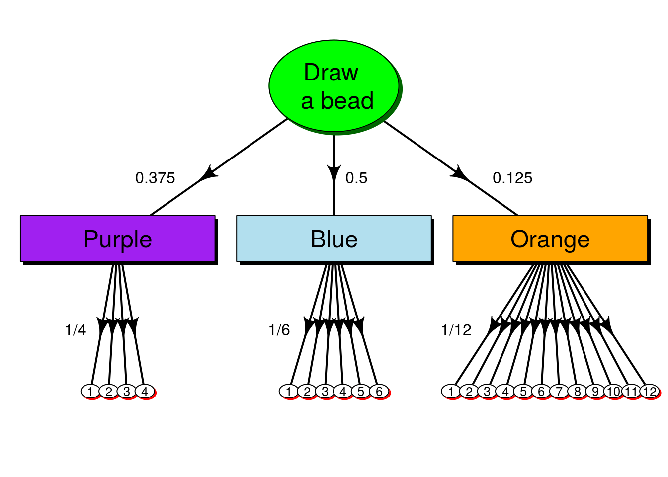
From this, we can calculate any of the probabilities we want. So, let’s calculate the probability of rolling a one. As above, we find all of the 1’s on the diagram, then multiply the probabilities to get to them. In notation, this is:
p(6) = p(purple) * p(1|purple) + p(blue) * p(1|blue) + p(orange) * p(1|orange)
Plugging in the numbers from the diagram (which match what we had above), we can get:
p(6) = 0.375 * 1/4 + 0.5 * 1/6 + 0.125 * 1/12
We can either type that (or copy-paste it) in R, like this:
# Use raw numbers
0.375 * 1/4 + 0.5 * 1/6 + 0.125 * 1/12
## [1] 0.1875Or, we can use the named probabilities that we saved before:
# Calculate in R
prob["purple"]   * 1/4 +
  prob["blue"]   * 1/6 +
  prob["orange"] * 1/12
## purple
## 0.1875Note that both give us exactly the same answer.
36.7.1 Try it out
Based on the following tree diagram, what is the probability that you will arrive at your destination early?
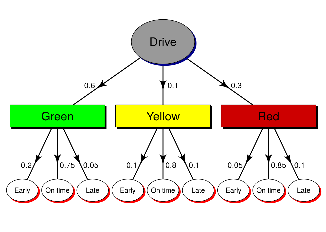
You should get 0.145.
36.8 What’s coming next
We have spilled a lot of pixels talking about conditional probabilities, focusing a lot on this idea expresed with the pipe (|) meaning: probability of something happening given that something else is true. That is a lot like the definition of the p-value: the probability of getting data as extreme as, or more extreme than, the observed data given that the null hypothesis is true.
This is not a coincidence. The p-value is explicitly a conditional probability. However, remember that the p-value only gives the probability of getting the data, not the probability that the null is true. In our last example with the stop lights, for example, we might say that being late will only occur 5% of the time that the light was green, so we reject our null hypothesis that the light was green.
However, that rejection doesn’t tell us how likely it was that the light actually was green. For that, we need to “reverse” the condition. Somehow, we need to get from the information that we have showing that the p(Late|Green) = 0.05 to a measure of p(Green|Late). For that, we will use something called Bayes Theorem – and the results may initially surprise you.