An introduction to statistics in R
A series of tutorials by Mark Peterson for working in R
Chapter Navigation
- Basics of Data in R
- Plotting and evaluating one categorical variable
- Plotting and evaluating two categorical variables
- Analyzing shape and center of one quantitative variable
- Analyzing the spread of one quantitative variable
- Relationships between quantitative and categorical data
- Relationships between two quantitative variables
- Final Thoughts on linear regression
- A bit off topic - functions, grep, and colors
- Sampling and Loops
- Confidence Intervals
- Bootstrapping
- More on Bootstrapping
- Hypothesis testing and p-values
- Differences in proportions and statistical thresholds
- Hypothesis testing for means
- Final thoughts on hypothesis testing
- Approximating with a distribution model
- Using the normal model in practice
- Approximating for a single proportion
- Null distribution for a single proportion and limitations
- Approximating for a single mean
- CI and hypothesis tests for a single mean
- Approximating a difference in proportions
- Hypothesis test for a difference in proportions
- Difference in means
- Difference in means - Hypothesis testing and paired differences
- Shortcuts
- Testing categorical variables with Chi-sqare
- Testing proportions in groups
- Comparing the means of many groups
- Linear Regression
- Multiple Regression
- Basic Probability
- Random variables
- Conditional Probability
- Bayesian Analysis
Shortcuts
28.1 Load today’s data
Start by loading today’s data. If you need to download the data, you can do so from these links, Save each to your data directory, and you should be set.
- icuAdmissions.csv
- Data on patients admitted to the ICU.
- classGrades.csv
- This gives the grade (in points) for several types of assessments in a class that I was peripherally involved in.
- Each row is a student.
- Lab quizzes are out of 5 points, exams are out of 100 points, and all other items are out of 10 points.
# Set working directory
# Note: copy the path from your old script to match your directories
setwd("~/path/to/class/scripts")

# Load data
icu           <- read.csv("../data/icuAdmissions.csv")
classGrades   <- read.csv("../data/classGrades.csv")
28.2 A massive shortcut
We have now reached the point in this tutorial where you are going to hate me for making you do extra work. Working through all of the examples up to now by hand is very important to make sure that you understand what is happening.
However, we have now reached a point where the data, and the questions, are starting to get complicated enough that doing them by hand is no longer possible. So, here, I introduce you to functions, already written for R, that do these calculations for you. You still need to understand what you are inputing, and what the outputs mean, but the detailed mechanics are no longer as necessary. This will also allow us to address more questions in less time, focusing on interpretations instead of mechanics.
28.3 The t-test
In R, the t-test (for means) is implemented as the function t.test(). This function takes data in a lot of different ways, and I will try to show the major ones here. If you are ever in doubt, make sure that the output makes sense, and check the help (?t.test) for more details. As always, it is a good idea to plot your data as well.
28.3.1 For single mean
In this section, we will be looking at the Age column from the icu data. So, let’s start by plotting it:
boxplot(icu$Age, ylab = "Age (years)")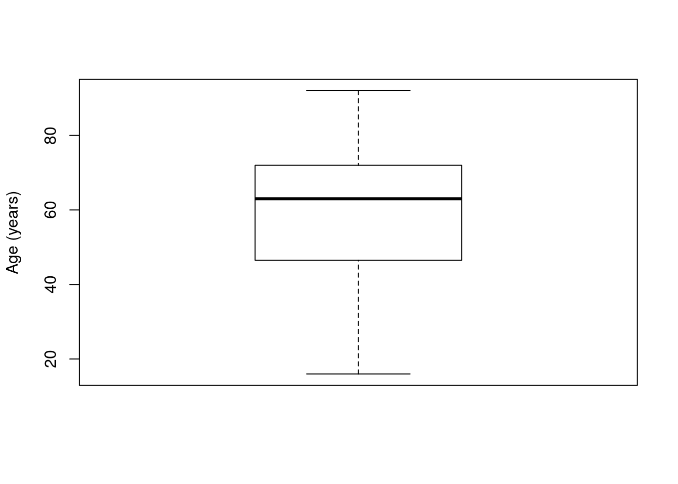
As when we started to use the t-distribution, the simplest use for the t-test is to test a single mean. For this, we simply give the function t.test() a numeric vector, such as the Age column from the icu data:
# Simple one sample t-test
t.test(icu$Age)
##
## One Sample t-test
##
## data: icu$Age
## t = 40.5796, df = 199, p-value < 2.2e-16
## alternative hypothesis: true mean is not equal to 0
## 95 percent confidence interval:
## 54.74861 60.34139
## sample estimates:
## mean of x
## 57.545This gives us a 95% confidence interval, which here means that we are 95% confident that the true mean age lies between 54.75 and 60.34 years old and tells us that the mean value is 57.55. This is based on exactly the same methods that we have been working with.
It also gives us a t-statistic, degrees of freedom, and a p-value. However, if you look at the alternative hypothesis you will note that it is testing whether or not the mean is 0. That is probably not a reasonable null hypothesis to have. Instead, we might have predicted that the mean was 60 (e.g., if that was the value at some other hospital). Thus, our H0 becomes that mean is equal to 60. We can test that mean by setting the argument mu = to our null (recall that mu, the Greek character μ, is the notation for the true population mean).
# Test a different alternate hypothesis
t.test(icu$Age, mu = 60)
##
## One Sample t-test
##
## data: icu$Age
## t = -1.7312, df = 199, p-value = 0.08496
## alternative hypothesis: true mean is not equal to 60
## 95 percent confidence interval:
## 54.74861 60.34139
## sample estimates:
## mean of x
## 57.545Note that our confidence interval did not change, but the t-statistic and p-value (and null hypothesis) did. The t-statistic is calculated the same way that we have been doing it by hand
\[ t = \frac{obs - H_0}{SE} \]
That is the difference between our observed data and the null hypothesis, divided by the calculated standard error (\(SE = \frac{s}{\sqrt{n}}\)). This gives us how different our data are from the null in number of standard errors. The function then calls pt() to determine how likely such a difference (or bigger) was to happen by chance.
Finally, we can also change the size of the confidence interval by setting the conf.level = argument to the size of our desired confidence interval. So, we can calculate a 90% confidence interval like this:
# Test a different alternate hypothesis
t.test(icu$Age, mu = 60, conf.level = 0.90)
##
## One Sample t-test
##
## data: icu$Age
## t = -1.7312, df = 199, p-value = 0.08496
## alternative hypothesis: true mean is not equal to 60
## 90 percent confidence interval:
## 55.20156 59.88844
## sample estimates:
## mean of x
## 57.545Of note, we can pass in any numeric vector, including the value for a subset. So, we could calculate the 90% confidence interval (and test the null hypothesis that the mean is 60 years old) for just women with the following:
# Use this on a subset of data
t.test(icu$Age[icu$Sex == "female"],
       mu = 60, conf.level = 0.90)
##
## One Sample t-test
##
## data: icu$Age[icu$Sex == "female"]
## t = 0, df = 75, p-value = 1
## alternative hypothesis: true mean is not equal to 60
## 90 percent confidence interval:
## 56.00834 63.99166
## sample estimates:
## mean of x
## 60We once again get a confidence interval, though this time our p-value is 1. That is because the observed mean is equal to the null hypothesis. However: that still does not mean that the null hypothesis is (necessarily) true. It only means that we cannot reject it.
28.3.1.1 Try it out
First, calculate a 99% confidence interval of the mean heart rate (column HeartRate). You should get an interval between 93.99 and 103.86 bpm.
Then, test the null hypothesis that the mean heart rate is 100 bpm. You should get a p-value of 0.572.
28.3.2 For difference in means
The function t.test() also works well for testing for a difference in means, such as between two groups. For this, let’s look at the Age column of icu split by Infection. As always, start by plotting your data.
# Show a box plot of the two groups
plot(Age ~ Infection, data = icu)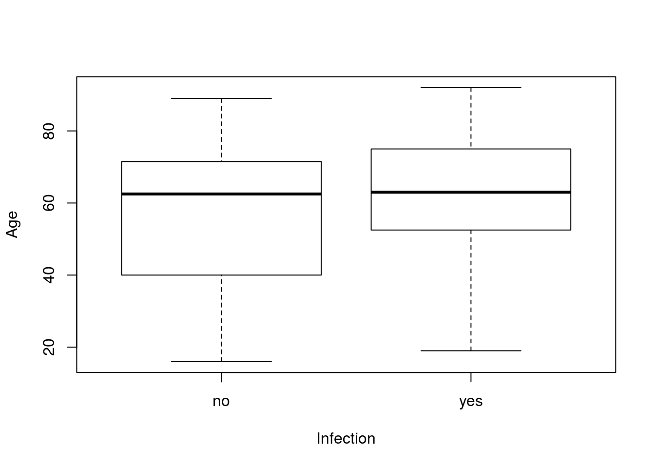
There looks to be a small, but not huge, difference between the two groups. We can test it using the t.test() function with the exact same arguments we used to plot the data. This is one of the benefits of the copy-paste approach: once you have plotted the data, you can just copy the line, replace plot with t.test and go.
# Run a t.test
t.test(Age ~ Infection, data = icu)
##
## Welch Two Sample t-test
##
## data: Age by Infection
## t = -2.2481, df = 193.601, p-value = 0.02569
## alternative hypothesis: true difference in means is not equal to 0
## 95 percent confidence interval:
## -11.6837808 -0.7636741
## sample estimates:
## mean in group no mean in group yes
## 54.93103 61.15476This gives us means of each group, the information for the test, and a confidence interval for the difference between the groups. One important note is the degrees of freedom. When doing these by hand, we were using one less than the smaller sample size. Here, the function instead uses the more complicated formula[*] The formula for the degrees of freedom is technically: \[
\frac{\left( \frac{s_1^2}{n_1} + \frac{s_1^2}{n_1} \right)^2}
{ \frac{\left( \frac{s_1^2}{n_1} \right)^2}{n_1 - 1} +
\frac{\left( \frac{s_2^2}{n_2} \right)^2}{n_2 - 1}
}
\] Hopefully it is clear why I hid it here. to calculate the degrees of freedom. That difference is why your answers from doing differences in means by hand will differ slightly from the answers given by t.test()
28.3.2.1 Plotting the difference better
Here, we see that we get a significant difference. However, our plot doesn’t show that very clearly. Instead, we would probably like to plot the means with confidence intervals. Recall from one of our very first chapters that we introduced the package gplots and the function plotmeans(). To use it, first load gplots:
library(gplots)If that gave you an error message, re-install the package with:
# ONLY RUN THIS IF YOU NEED TO RE-INSTALL
install.packages("gplots")
Now, we can use plotmeans, which again takes almost exactly the same arguments as t.test() and plot()
# Plot the data with confidence intervals
plotmeans(Age ~ Infection, data = icu)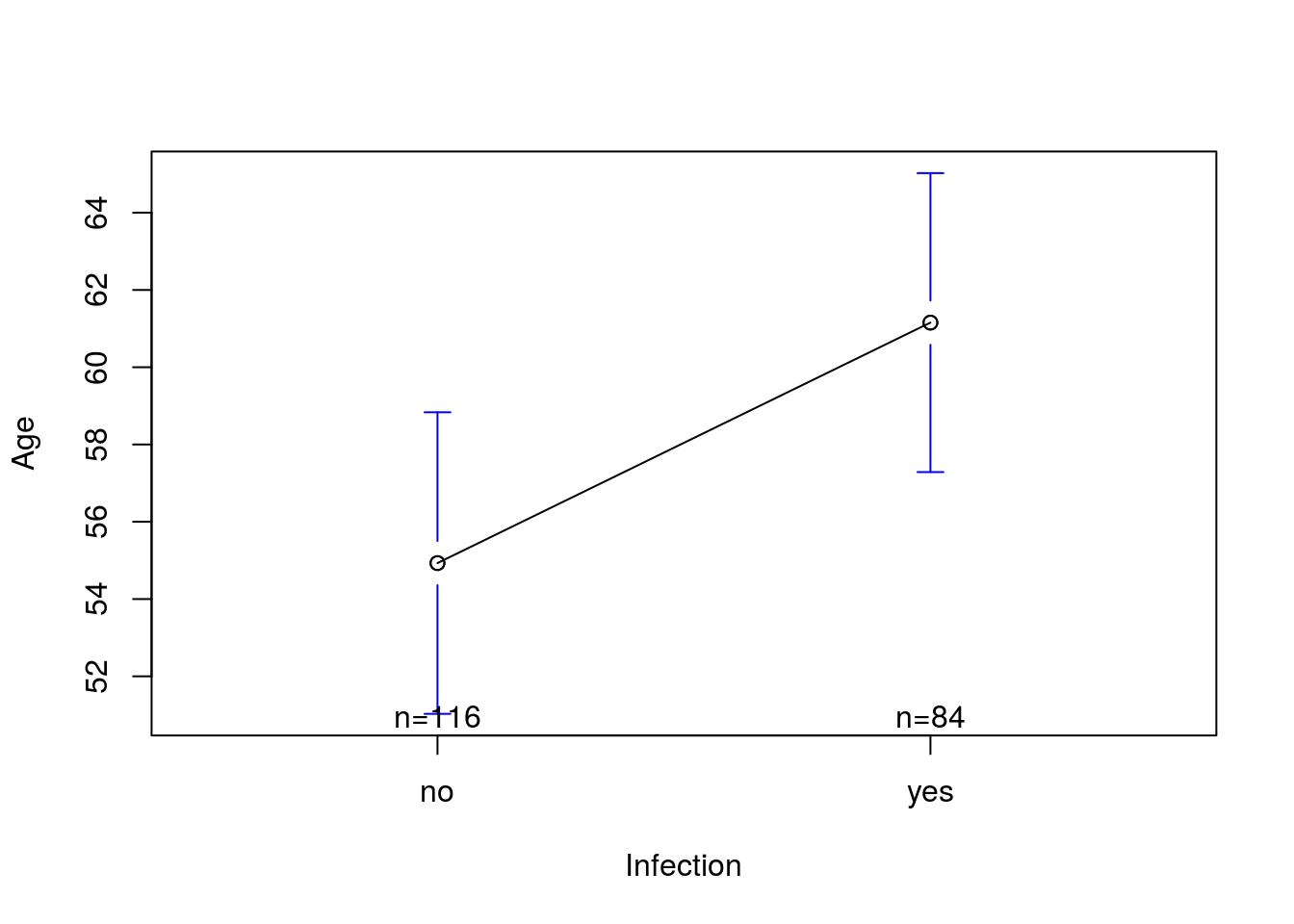
Here, each group is plotted with a 95% confidence interval. Those confidence intervals are what you would calculate for each group separately. They are a good visual indication, though do not match perfectly to the p-value given by a t-test, in part because of differences in degrees of freedom.
Personally, I like to clean up the output of plotmeans() a little bit. My preference is to keep the plot simple, with fewer labels. So, I usually add n.label = FALSE to not print the sample sizes and connect = FALSE to not draw a line between the two groups.
plotmeans(Age ~ Infection, data = icu,
          n.label = FALSE, connect = FALSE)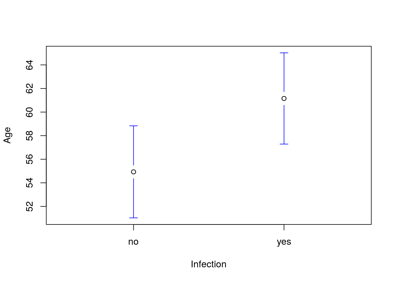
For more control, see the help (?plotmeans) for a long list of options that you can control, including being able to set a different size for the confidence interval. If you want even more control (such as to add the error bars to a different plot) check out the function plotCI(), which is what plotmeans() is calling to do the final plotting (it just handles calculating means and CI’s for you first).
28.3.2.2 Handling multiple levels
Finally, this approach is especially nice if we want to exclude some of our observations, as we will see in a moment. What if I want to see the difference in Age between levels of Consciousness? Let’s try it:
# t.test for server's tips
t.test(Age ~ Consciousness,
       data = icu)
## Error in t.test.formula(Age ~ Consciousness, data = icu): grouping factor must have exactly 2 levelsNote that we get an error – the t-test only works with two groups, and there are three levels in Consciousness. We will see how to deal with more groups in a coming chapter, but for now, we just need to stick to pairwise comparisons. Luckily, with the data = argument, it is easy to exclude the one we don’t want or include only those we do:
# t.test for Age by Consciousness with out deepStupor
# don't forget the comma to say we are talking about rows
t.test(Age ~ Consciousness,
       data = icu[icu$Consciousness != "deepStupor",])
##
## Welch Two Sample t-test
##
## data: Age by Consciousness
## t = 1.9803, df = 11.797, p-value = 0.07148
## alternative hypothesis: true difference in means is not equal to 0
## 95 percent confidence interval:
## -0.8575128 17.6142696
## sample estimates:
## mean in group coma mean in group conscious
## 65.40000 57.02162That looks a bit better. Of note, instead of excluding “deepStupor”, we could also have only included the two values we wanted (e.g if there are lots of levels).
# t.test for Age by Consciousness with only coma and conscious
# don't forget the comma to say we are talking about rows
t.test(Age ~ Consciousness,
       data = icu[icu$Consciousness == "coma" |
                  icu$Consciousness == "conscious",])
##
## Welch Two Sample t-test
##
## data: Age by Consciousness
## t = 1.9803, df = 11.797, p-value = 0.07148
## alternative hypothesis: true difference in means is not equal to 0
## 95 percent confidence interval:
## -0.8575128 17.6142696
## sample estimates:
## mean in group coma mean in group conscious
## 65.40000 57.02162The outputs are identical, and we can use this approach for any similar question. In addition, we could also ask if there is any difference between those coded as “coma” and any other value. For this, we simply use the == to get “TRUE” and “FALSE” for the column of interest.
t.test(Age ~ Consciousness == "conscious",
       data = icu)
##
## Welch Two Sample t-test
##
## data: Age by Consciousness == "conscious"
## t = 2.0466, df = 21.538, p-value = 0.05309
## alternative hypothesis: true difference in means is not equal to 0
## 95 percent confidence interval:
## -0.1017174 14.0584742
## sample estimates:
## mean in group FALSE mean in group TRUE
## 64.00000 57.02162So, “TRUE” are patients coded as “conscious” and “FALSE” is all other codings. This is especially helpful when we are trying to compare one group against the rest of the possible values. As always, don’t forget to plot your results:
# Plot the full result
plotmeans(Age ~ Consciousness,
          data = icu,
          n.label = FALSE, connect = FALSE)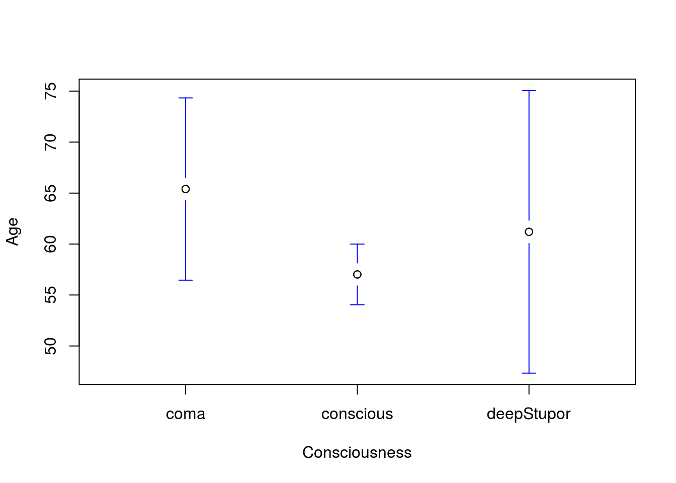
Note that this plot shows all three groups. In the coming weeks we will be able to analyze all of the groups. And the result of just “conscious” compared to all of the others:
# Plot the full result
plotmeans(Age ~ Consciousness == "conscious",
          data = icu,
          n.label = FALSE, connect = FALSE)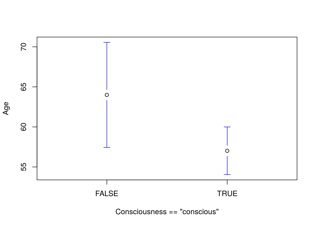
We can also fix up the labels. In this function legends = is the argument to change the labels on the x-axis (I usually have to look in the help everytime I want to use that).
# Plot the full result
plotmeans(Age ~ Consciousness == "conscious",
          data = icu,
          legends = c("not conscious","conscious"),
          xlab = "Conscious State",
          n.label = FALSE, connect = FALSE)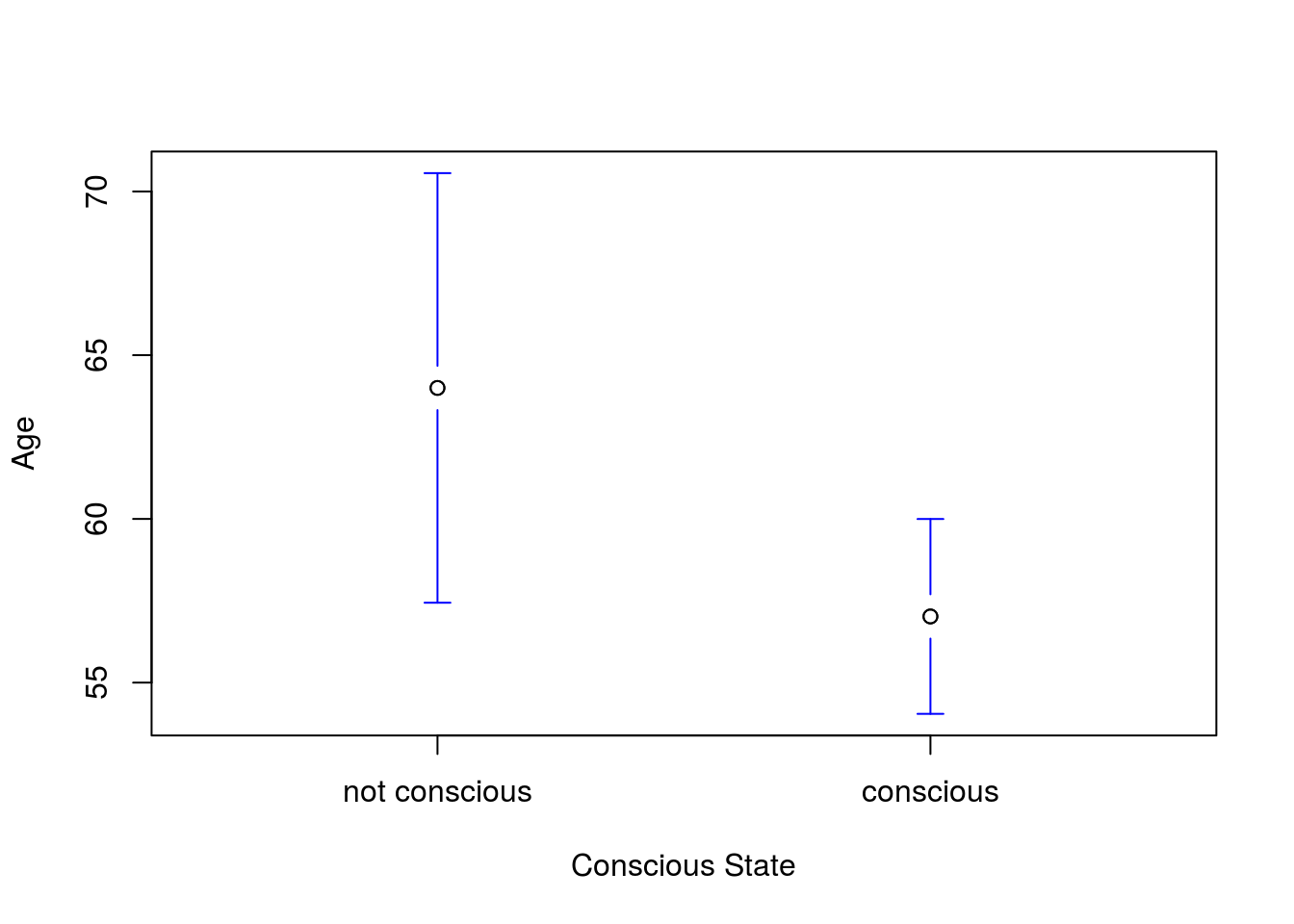
28.3.2.3 Try it out
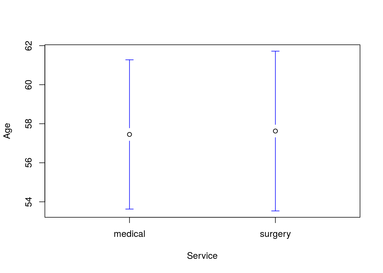
Run a t-test for a difference in the mean Age by Service and include a plot. You should get a p-value of 0.951 and a plot like this:
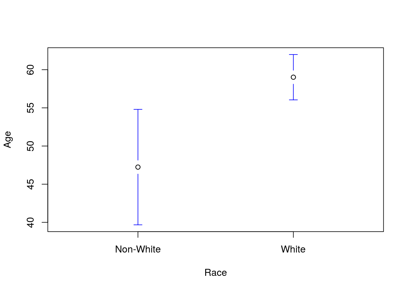
Then, run a t-test for a difference in Age between patients coded as “white” and all other groups. You should get a p-value of 0.0055 and a plot like this:
28.3.3 Paired data
Our final approach for t.test() will be to assess paired variables. For this, we will compare lab quiz 6 (column labQuiz06) against the lecture quiz 3 (column classQuiz03) from the classGrades data.
This will require some extra manipulation as the lab quizzes are out of 5 points, and the class quizzes are out of 10 points. To handle this, we will represent each as a percentage score and save them in their own variable.
# Store the variables
labQ <- classGrades$labQuiz06 / 5
lecQ <- classGrades$classQuiz03 / 10
We can then plot those scores:
boxplot(labQ, lecQ,
        names = c("lab","lecture"),
        xlab = "Quiz type",
        ylab = "Percent score")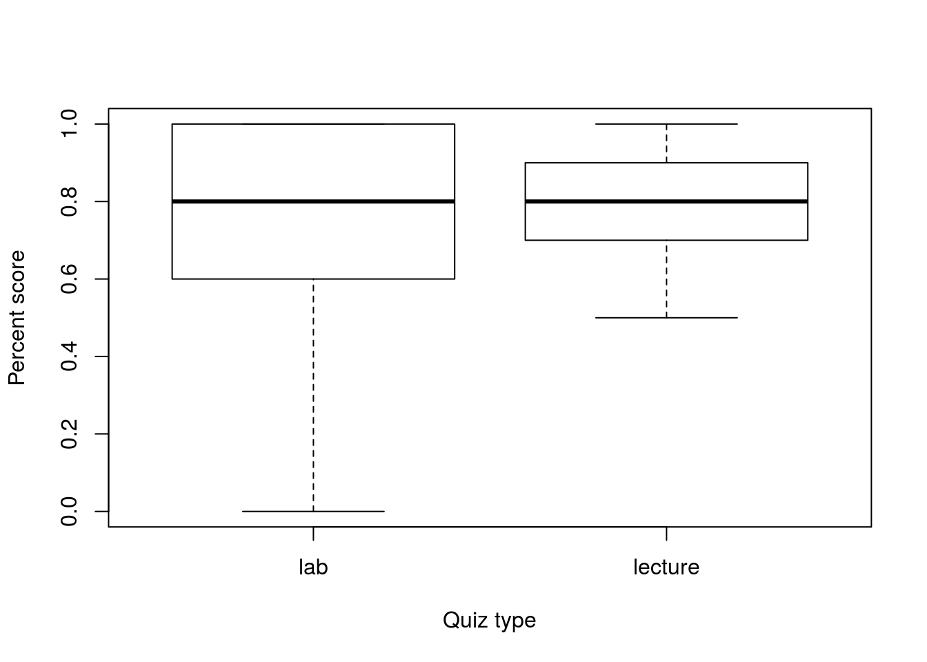
Now, we can use t.test() very similarly to boxplot() and pass in two vectors of data. t.test() will then compare them against each other.
# Run a t.test
t.test(labQ, lecQ)
##
## Welch Two Sample t-test
##
## data: labQ and lecQ
## t = -1.6932, df = 37.23, p-value = 0.09877
## alternative hypothesis: true difference in means is not equal to 0
## 95 percent confidence interval:
## -0.22808939 0.02039708
## sample estimates:
## mean of x mean of y
## 0.7076923 0.8115385But, if you recall from our earlier chapter, we know more about these data. Specifically we know that they are paired. To handle this with the t.test() function, we add the argument paired = TRUE.
# Run paired t.test
t.test(labQ, lecQ, paired = TRUE)
##
## Paired t-test
##
## data: labQ and lecQ
## t = -2.0999, df = 25, p-value = 0.04599
## alternative hypothesis: true difference in means is not equal to 0
## 95 percent confidence interval:
## -0.205695742 -0.001996566
## sample estimates:
## mean of the differences
## -0.1038462Now that is what we had in our previous chapter. This makes it easy to handle paired data, but we still need to remember when it is appropriate. One good rule of thumb is to always try to use the formula approach if possible. If it is not possible, think about why that is the case and you will often (though not always) find that it is because your data are paired measures of different things, rather than a measure of one thing separated by another variable that groups them.
28.3.3.1 Try it out
Run a test to compare lab quiz 7 and lecture quiz 6? Make sure to state your hypotheses and run an appropriate test. Don’t forget that the lab quiz is out of 5 and the lecture (class) quiz is out of 10 (Like I did when I first calculated the value to put here).
You should get a p-value of 0.174.
28.3.4 (Not) Working from summary data
Perhaps unfortunately, the t.test() function does not provide a means to work from summary data. This is, perhaps, because the need is rare outside of intro stats courses, or perhaps becuase of the simplicity of the calculations. In either case, to work from summary data, you will have to continue working the problems by hand. Alternatively, you could write a function of your own to handle summary data for t-tests. The choice is yours.
28.4 The proportion test
Just like for the t-test, R has a built in function to handle tests of proportions. I am less familiar with this test, so if there is something you think it should be able to do, check the help with ?prop.test.
Unlike t.test(), the function prop.test() works on summary data, so we still need to either use sum() to count our successes and length() or nrow() to count our trials, or to use table() to supply all of the needed values. but it will then do much of the rest of the work.
28.4.1 One sample
For a one-sample test, we just give it our successes and trials, along wtih a null hypothesis. So, if we want to test whether or not the proportion of female patients in the ICU is 0.5 (a null that assumes equal numbers of men and women), we would use the following. Note that this treats the first “level” of the table as the “successes”, so we are given an estimate (and confidence interval) for the proportion of female patients. Make suree that you are aware of this when using this tool.
# View data
table(icu$Sex)
##
## female male
## 76 124# Run one sample test
prop.test(table(icu$Sex), p = 0.5)##
## 1-sample proportions test with continuity correction
##
## data: table(icu$Sex), null probability 0.5
## X-squared = 11.045, df = 1, p-value = 0.0008893
## alternative hypothesis: true p is not equal to 0.5
## 95 percent confidence interval:
## 0.3132213 0.4514680
## sample estimates:
## p
## 0.38This returns a p-value showing that, with a small value, we can reject the null hypothesis that 50% of patients are male. It also gives us 95% CI. As with t.test() we can change the interval of that CI with conf.level =:
# Get a 90% CI instead
prop.test(table(icu$Sex),
          conf.level = 0.9)
##
## 1-sample proportions test with continuity correction
##
## data: table(icu$Sex), null probability 0.5
## X-squared = 11.045, df = 1, p-value = 0.0008893
## alternative hypothesis: true p is not equal to 0.5
## 90 percent confidence interval:
## 0.3231067 0.4402375
## sample estimates:
## p
## 0.38Note the change in confidence level, showing u the 90% level. In addition note that, by not setting p =, it defaults to 0.5.
28.4.1.1 Try it out
Calculate a 99% confidence interval for the true proportion of patients that did not have a previous visit (column Previous is “no”).
You should get an interval of 0.771 to 0.9057.
28.4.2 Two samples
What if we want to compare two groups, like testing to see if “medical” and “surgery” Service have the same proportion of men and women? First, let’s look at our data.
# Look at the data
table(icu$Service, icu$Sex)
##
## female male
## medical 39 54
## surgery 37 70So, our assumptions are met (at least ten in each count). We may want to manually check the proportions too. this is a good idea, especially when using a new test as it gives you a good double-check of the output values.
# Check proportion in each service
prop.table(table(icu$Service, icu$Sex), 1)
##
## female male
## medical 0.4193548 0.5806452
## surgery 0.3457944 0.6542056Now, we can use this table to run our test.
# run the test
prop.test(table(icu$Service, icu$Sex))
##
## 2-sample test for equality of proportions with continuity
## correction
##
## data: table(icu$Service, icu$Sex)
## X-squared = 0.8518, df = 1, p-value = 0.356
## alternative hypothesis: two.sided
## 95 percent confidence interval:
## -0.07132024 0.21844113
## sample estimates:
## prop 1 prop 2
## 0.4193548 0.3457944Note that the estimates follow the order in the table. Specifcally, the left column is the “successes” (here, being “female” because it is first alphabetically), and the proportions are in the same order as the rows (medical then surgery). If you were ever unsure of this, using the table of proportions above can be especially helpful.
As with the t.test(), this value very nearly matches what we previously calculated by hand. It is using a slightly different statistic, designed to handle more than two groups, which we will explicitly discuss in a chapter very soon.
28.4.2.1 Try it out
Run a test comparing the proportion of patients that live or die by sex. That is, is there a differnce in the probability of survival by sex?
You should get a p-value of 0.913
28.4.3 Entering data from summary
Often, especially when given data for problems in an intro stats course, we are given counts instead of raw data to work with. In this case, we can use prop.test() in a slightly different way. First, let’s consider our tie example from earlier chapters:
President Artman recently started wearing a new tie. You are interested in knowing how students are responding, particularly whether men and women are responding differently. Instead of asking every student on campus, you surveyed a random subset of students (a good, representative sample). In this survey, you asked each student if they “loved” or “hated” the new tie. Your results: 57 men loved it, 41 men hated it; 227 women loved it, 78 women hated it.
Now, for prop.test() we need to submit the two success numbers (number of each sex that loved the tie) as a vector, and the two total trials (total number of each sex) as a separate vector. Therefore, we can enter our data as
# Run two sample test
prop.test( c(57    , 227),
           c(57+41 , 227+78))
##
## 2-sample test for equality of proportions with continuity
## correction
##
## data: c(57, 227) out of c(57 + 41, 227 + 78)
## X-squared = 8.6615, df = 1, p-value = 0.00325
## alternative hypothesis: two.sided
## 95 percent confidence interval:
## -0.27862164 -0.04663765
## sample estimates:
## prop 1 prop 2
## 0.5816327 0.7442623