An introduction to statistics in R

A series of tutorials by Mark Peterson for working in R

Chapter Navigation

34.1 Load today’s data

No data to load for today’s tutorial. Instead, we will be using R’s built in randomization functions to generate data as we go.

34.2 Background

There are a lot of phenomena that we often think of as “random.”

Will the light be green when I get to the interesction?
Will this die land “six” when I roll it?
Will I draw a white bead from the bag in the next draw?

Now, these phenomena may be random, but that doesn’t mean that we know nothing about them. We may know that the light is green more often for cars going North/South than for cars going East/West. We may know that the die has six sides, each of which are equally likely to land up. We may have observed how often white beads have appeared already.

Each of these things tells us something about the probability of an event occurring. The last example (about green beads) gives us a formal definition to use:

Probability

The frequency of an event occurring over many trials.

If we have observed 100 draws, and 53 of them have been white beads, we might say that we think the probability of drawing a white bead is 0.53 (or 53%). The confidence intervals we have been calculating throughout the tutorial could give us information about how sure we are about that, but over a large enough number of draws, we know that the confidence interval will get very, very small.

We call each event (draw, roll, flip, arriving at the light, treating a patient, etc.) a “trial” and record the result as the “outcome” (white, blue, four, five, green light, red light, live, die, get better, etc.). For any given trial there are a fixed number of possible outcomes called the “sample space.” The total probability of the sample space has to equal 1, as one of the outcomes must occur. So, for our bead example, if our probability getting a white bead is 0.53, our probability of getting “not white” is 0.47.

34.2.1 Theoretical probability

Sometimes, we may be able state the probability before we observe any trials. This is generally referred to as theoretical probability (as opposed to the empricial probality described above), and is perhaps more common to everyday thinking. In the die example, we are likely confident in saying that the probability of rolling a six on a fair six-sided is one-in-six (\(\frac{1}{6}\) = 0.1667). We can say this without having observed any trials because we know something about the system.

That doesn’t mean that the probability always has to be fair. Instead, we could base it on some knowledge of the system. For example, we may know the city manager responsible for setting the stop lights, and know that ze set the lights to be green on the north-south direction 60% of the time. Our probability of hitting a green at that intersection when driving north or south is then 0.6.

All of these approaches to probability work the same in the end. What we will be doing in this chapter is using those calculated or theorized probabilities to say larger things about the way probability works.

34.3 A simple example

Let’s start by generating a set of simple beads. Imagine that we are putting 20 beads in a cup:

4 black
2 blue
8 orange
6 white

We can simulate that in R using rep(), like we have before:

# create the bead cup
beads <- rep(c("black","blue","orange","white"),
             c(   4   ,   2  ,   8    ,   6   ))
table(beads)

black	blue	orange	white
4	2	8	6

We can then simulate drawing from the this cup (with replacement) a large number of times using sample()

# Draw a bunch of beads
sampledBeads <- sample(beads,
                       size = 2036,
                       replace = TRUE)
# See the results
table(sampledBeads)

black	blue	orange	white
404	204	817	611

Hopefully unsurprisingly, those ratios look very similar to our starting values (yours will obviously be a little different). We can check the proportions directly:

round(table(sampledBeads) / length(sampledBeads),3)

black	blue	orange	white
0.198	0.1	0.401	0.3

round(table(beads) / length(beads),3)

black	blue	orange	white
0.2	0.1	0.4	0.3

We can then simulate drawing from the this cup (with replacement) a large number of times using sample()

# Draw a bunch of beads
sampledBeads <- sample(beads,
                       size = 2036,
                       replace = TRUE)
# See the results
table(sampledBeads)

black	blue	orange	white
393	234	787	622

Hopefully unsurprisingly, those ratios look very similar to our starting values (yours will obviously be a little different). We can check the proportions directly:

round(table(sampledBeads) / length(sampledBeads),3)

black	blue	orange	white
0.198	0.107	0.393	0.302

round(table(beads) / length(beads),3)

black	blue	orange	white
0.2	0.1	0.4	0.3

So, we see that the proportions are converging to very near the expected distribution – just like our formal definition of probability.

34.3.1 An alternative data entry

The way we just entered these above was relatively straightforward for this small set. However, in more complicated situations, or with more precise probabilities, it is cumbersome. Instead, if we remember that sample() offers the p = argument, we might prefer to save our arguments in a different way.

Here, we can save a simple vector of the colors, and a separate vector of the probabilities. This approach is more scalable, and often more tractable. For the probabilities, you can either enter the probabilities directly (e.g. c(0.2, 0.1, 0.4, 0.3)) or caluclate them from relative probabilities (like the number of beads we have of each color) as I do below. This will ensure that the probabilities always sum to exactly one.

# Save bead colors
beadColor <- c("black","blue","orange","white")

# Save probabilities
prob <- c(4, 2, 8, 6)
prob <- prob / sum(prob)

# See them together
cbind(beadColor, prob)

beadColor	prob
black	0.2
blue	0.1
orange	0.4
white	0.3

We can then pass p = prob into sample() and it will appropriately balance the colors:

# Draw a bunch of beads
sampledBeads <- sample(beadColor,
                       size = 2036,
                       replace = TRUE,
                       p = prob)

# View proportions
round(table(sampledBeads) / length(sampledBeads),3)

black	blue	orange	white
0.201	0.106	0.382	0.311

This has the added benefit of having the probability directly saved as a vector, which we will utilize a lot as we continue with these calculations.

34.3.2 Try it out

Create a vector of traffic light colors and give them the following probabilities. (take care to not overwrite the prob and sampledBeads variables, as they will be used again soon).

trafficLights	probLight
red	0.3
yellow	0.1
green	0.6

Sample at least 2,000 trials (arrivals at the light) to see what proportion of the time you hit each color.

34.4 Simple addition

Often we may want to know the probability of getting either of two (or more) values. For example, we may want to know the probability of getting either a black or a blue bead.

For simple cases where we can never get both, we call these probabilities “disjoint” which means that you can only ever get one of the other. In the bead example, this is clear: any bead we draw can be either black or blue, but never both.

34.4.1 Simulation

Before we do the math, let’s see the result from our simulation. Looking at our table:

black	blue	orange	white	Sum
409	216	777	634	2036

We can quickly see that there are 409 black and 216 blue beads in our sample, for a total of 625 black or blue beads. We could then divide by the total number of beads to get a probability of getting either of these colors of \(\frac{625}{2036}\) = 0.307.

However, we can also test it directly from the vector of results. This may seem more complicated, but (as is often the case) it will make things easier soon. For this, we will ask for each bead if it is either black or (using the | pipe character) blue.

# Get true/false for each sampled bead
isBlackOrBlue <- sampledBeads == "black" | 
                 sampledBeads == "blue"

# See the results
table(isBlackOrBlue)

## isBlackOrBlue
## FALSE  TRUE 
##  1411   625

We can then either get just the number of TRUE’s with sum() or the proportion (what we are interested in) with mean() (it counts up the TRUE’s as 1’s and then divides by the number of sampled beads).

# Get proportion
mean(isBlackOrBlue)

## [1] 0.3069745

This works well for a small number of colors, but you can imagine that if we wanted to know if it matched one of ten (or even more) colors, that there would be a lot of redundant typing. Instead, R offers us the operator %in% which, like the == with | approach returns TRUE’s and FALSE’s. However, instead of asking if there is a match to just one color with each ==, we can ask if each bead matches anything in the list we give it. We can combine this with mean() directly, and get the same result as above.

# Calculate proportion black or blue directly
mean(sampledBeads %in% c("black","blue"))

## [1] 0.3069745

This approach is just collapsing all of those | into one statement, which can help keep code clean and avoid typos.

34.4.2 The math

While the additional logic approaches to show how to caluclate the proportion from our sample are helpful for working from simulations, it is the first approach that is most informative for doing the math. When we first looked at the table of results:

black	blue	orange	white	Sum
409	216	777	634	2036

it was intuitive to simply add up the two results we were interested in. We want to know the blues and the blacks, so just add them up. It is no more complicated here. Because the probabilities are disjoint (non-overlapping, i.e., we can’t get both blue and black), we can simply add them together, just like we intuitively want to.

For this, I find it helpful to name the vector of probabilities:

# Name the probabilities
names(prob) <- beadColor
prob

	black	blue	orange	white
prob	0.2	0.1	0.4	0.3

Now, just like above with the counts, we can add up the probabilities. Because the whole already sums to one (by definition), we don’t need to worry about dividing to get a probability. We could type in the numbers:

# Calculate the probability of either color
0.2 + 0.1

## [1] 0.3

This very similar to the result we got from our simulation,

However, if something changes (e.g., we set up a new cup) we might forget to change it. Instead, I prefer to use sum() and add up the probabilities that I want:

# More programatic way to calculate
sum(prob[c("black","blue")])

## [1] 0.3

34.4.3 Try it out

Generally speaking, I don’t stop for yellow lights. So, for my driving, I usually want to know what the probability is that the light will be either yellow or green when I reach it. Use the numbers from the last try it out to calculate the probability that the light will be either yellow or green.

(You should get 0.7.)

34.5 Combining two events

The above works great for disjoint outcomes, but what about when we are interested in the outcome of two events. We might want to know the probability is that the Vikings will win and that the Packers will lose. In this case, we can’t simply add because it is possible for the Vikings to win and the Packers to lose (it is the outcome we are interested in). When the two events don’t impact each other (e.g. the Vikings winning won’t affect the outcome of the Packers game) we call the events “Independent.”

With independent events, we can ask about the probability of both occurring. These events could be similar (e.g. two football games) or separate. As a clearer example of the latter, we can imagine rolling a die after we draw a bead. For the purposes here, let’s say that we are interested in the probability of getting a black bead and rolling a 1. For simplicity, we will assume we have a fair six-sided die.

34.5.1 Simulation

As always, we can start with a simulation to see what we are looking at. Because the die roll is independent of the bead color, we simply sample the same number of rolls as we have beads.

diceRolls <- sample(1:6,
                    size = length(sampledBeads),
                    replace = TRUE)

# See results
table(diceRolls)

1	2	3	4	5	6
327	345	335	348	328	353

As expected, we get a fairly even distribution of values from the dice. We can see what the first 6 trials would have looked like:

cbind(trial = 1:6,
      color = sampledBeads[1:6],
      die = diceRolls[1:6]
      )

trial	color	die
1	orange	4
2	orange	3
3	black	3
4	white	1
5	white	2
6	white	5

So, now, we want to know the probability of getting both a black bead and a 1. We can see this by making a table of the results:

addmargins( table(sampledBeads, diceRolls) )

	1	2	3	4	5	6	Sum
black	66	60	69	74	67	73	409
blue	33	45	30	42	34	32	216
orange	129	135	137	121	122	133	777
white	99	105	99	111	105	115	634
Sum	327	345	335	348	328	353	2036

We can quickly see that we got 66 black beads with 1’s. Dividing by the total gives us a proportion of 0.032. But - how can we get there with out a big simulation?

34.5.2 The math

In this case, the arithmetic is as simple as before, though the thought process may be less intuitive. Imagine that you just drew a black bead, what is the probability now of rolling a 1?

It is still \(\frac{1}{6}\), just like it would be if we had drawn another color. So, we know that of the times we draw a black, \(\frac{1}{6}\) of them will also roll a 1. Well, we also know that the probability of drawing a black is 0.2. So, 20% of the time we roll a 1, we will get a black bead. To combine these, we simply multiply the two probabilities.

The probability of getting both of any two indepent outcomes is the product of their probabilities (i.e., their probabilities multiplied). For our example, that means we can do this:

# Calculate probability of black and 1
prob["black"] * 1/6

##      black 
## 0.03333333

Which is very, very close to the value we observed in the simulation. However, note that this only works when the two events are independent. In the next chapter, we will explore some limitations to this rule.

34.5.3 Combining similar events

While the above is a great example to work with, we usually want to know the probability of similar events. So, we might want to know the probability of drawing two white beads. For that, we use the exact same approach: we multiply the two probabilities:

# Probability of two white beads
prob["white"] * prob["white"]

## white 
##  0.09

Near the end of this chapter, we will explore events like this in greater depth.

34.5.4 Try it out

Imagine two scenarios, and calculate the probability of each. First, assuming that two traffic lights on your route each have the same probability of being green and are independent (e.g. they are not timed to sync up), what is the probability of hitting a green light on each? Second, imagine that after the stop light, there is a traffic circle where you need to come to a complete stop about 10% of the time. What is the probability of hitting a red light, then having to stop at the traffic circle?

(You should get 0.36 and 0.03 respectively)

34.6 General addition

What if, instead of being interested the Vikings winning and the Packers losing, we want to know how likely it is that the Vikings will win or the Packers will lose (e.g., either one will clinch a playoff spot). Or, what if you need either a Jack or a Spade to win a hand of poker?

These cases are not disjoint, as we could have both a Vikings win and a Packers loss, or we could draw the Jack of Spades. So, we can no longer simply add things together. Situations like this arise often, and require some special treatment.

Let’s return to our bead and die example to illustrate the point. Instead of asking the probablity of getting both a black bead and a 1, we want to know the probablity of getting either a black bead or a 1.

34.6.1 Simulation

As before, to ground truth our results, let’s look at the simulation results first.

addmargins( table(sampledBeads, diceRolls) )

	1	2	3	4	5	6	Sum
black	66	60	69	74	67	73	409
blue	33	45	30	42	34	32	216
orange	129	135	137	121	122	133	777
white	99	105	99	111	105	115	634
Sum	327	345	335	348	328	353	2036

We see that in 409 trials we got a black bead, and in 327, we got a 1 on the roll. If we add them together, we get 736. However, if we test this directly, we see a different answer:

sum(sampledBeads == "black" | diceRolls == 1)

## [1] 670

Only 670 of the trials had either a black or a 1. that is 66 more than we got when adding above. How might we figure out how much to remove, without having to run the simulation?

Notice that 66 is also the number of times that we get a trial with both a black bead and a 1. In fact, that is exactly the issue. When we took the row and column totals above, we counted that 66 twice! If we subtract it from our total, we get the correct answer:

sum(sampledBeads == "black") + sum(diceRolls == 1) -
  sum(sampledBeads == "black" & diceRolls == 1)

## [1] 670

If we use mean() (to get proportions) instead of sum() to get counts, we can get the correct total proportion too:

# Calculate the proportion that are either
mean(sampledBeads == "black") + mean(diceRolls == 1) -
  mean(sampledBeads == "black" & diceRolls == 1)

## [1] 0.3290766

and compare that to the direct calculation:

mean(sampledBeads == "black" | diceRolls == 1)

## [1] 0.3290766

34.6.2 The math

As we have seen throughout, any math or arithmetic that works on the counts in the simulation will also work on the probabilities. Here, we use the multiplication trick from above to calculate the probability of getting both, then subtract that from the sum of the two probabilities. (That is, we add the two probabilities, then substract the overlap to avoid counting it twice.)

# Calculate the probability of either
prob["black"] + 1/6 - (prob["black"] * 1/6)

##     black 
## 0.3333333

As before, this comes very, very close to our observed result, exactly as it should.

34.6.3 An additional step

As before, this approach can also work on independent trials of the same type of variable. For example, imagine that you are playing Yahtzee, and need a 5 on one of the next two rolls to make a Yahtzee (you rolled 4 fives on your first roll).

What is the probability that you will not roll a 5? (You are a pessimist, apparently.)

You could do some complicated calculations, but it is a lot easier to realize that the question is just asking “What is 1 - the probability of getting a 5 on roll one or roll two?”

So, we start by calculating the probability of getting at least one 5:

1/6 + 1/6 - (1/6 * 1/6)

## [1] 0.3055556

Our probability of rolling at least one five is 0.306. Because the total sample space has to add up to one (by definition), we know that this means our probability of not rolling a 5 is:

1 - (1/6 + 1/6 - (1/6 * 1/6))

## [1] 0.6944444

This also a good place to remind you about why the subtraction is necessary. If you roll six dice, are you definitely going to get at least one 5? Of course not – but if you just added up \(\frac{1}{6}\) six times, you would get a probability of one. Just another way to help remember that the subtraction is necessary.

34.6.4 Try it out

What is the probability of hitting a green light on either your first or second light?

(0.84)

What is the probability of either hitting the first light green or the second light yellow?

(0.64)

34.7 Binomial events

Binomial trials are cases in which we are only interested in the probability of “success” or “failure” of some trial – we are always limited to two outcomes (like when we did proportion tests). So, we need to set a new probability – lets call it probSuccess. For this example, let’s say that there is a 40% chance that, when playing a game, you get any points (though several different amounts of points may be possible).

# Set our probability of success
probSuccess <- 0.4
probSuccess

## [1] 0.4

Recall that this means, by definition, that the probability of “failure” is 1 - probSuccess (0.6) . What we are interested in now is how many times, given that probability and a certain number of trials, we are likely to get a success (get any points, in this case).

34.7.1 Simulation

There are a lot of ways to simulate binomial trials, but we are going to stick with a simple one for now. To simulate a single binomial process, we can just use sample. Here, we will set the variable n to be our number of trials (that is convention for the sample size).

# Set number of trials
n <- 3

# Simulate a single series of binomial trials
trials <- sample(c("points","no points"),
                 size = n,
                 replace = TRUE,
                 prob = c( probSuccess, 1 - probSuccess)
                 )
trials

## [1] "points" "points" "points"

Then, because we are interested in counting our successes, we can use sum() and a logical test (==) to see how many successes we got in our 3 trials.

# Count successes
sum(trials == "points")

## [1] 3

Here, we got 3 successes in 3 trials (note your values are likely different). We can do that in a for loop rather easily. Let’s see how many players get any points in three trials (e.g. attempts) when we do this many, many times:

# initialize variable to hold number of successes
nSuccess <- numeric()

for(i in 1:12345){
  trials <- sample(c("points","no points"),
                   size = n,
                   replace = TRUE,
                   prob = c( probSuccess, 1 - probSuccess)
                   )
  
  nSuccess[i] <- sum(trials == "points" )
}

# View results
table(nSuccess)

0	1	2	3
2667	5348	3551	779

This shows us that in our simulations, 5348 of the simulations had exactly one success. We will use this simulation result in a bit to test our calculations.

34.7.2 Probability of a particular sequence

When considering the probability of a particular sequence, we return to the basic rules of probability. Because each trial is independent, we can multiply the probabilities to get the probability of that full sequence.

For example, the probability of getting an order of: success, success, failure is:

# Calculate p of this sequence
probSuccess * probSuccess * (1 - probSuccess)

## [1] 0.096

Because there are only two probabilities there, we can simplify this by using exponents:

# Calculate p of this sequence
probSuccess^2 * (1 - probSuccess)^1

## [1] 0.096

If we call our number of successes in the sequence k we can make this easier to change

# Set number of trials and success
n <- 3
k <- 2

# Calculate p of this sequence
probSuccess^k * (1 - probSuccess)^(n - k)

## [1] 0.096

This shortcut will come in handy soon.

34.7.3 Probability of k successes

So, does that mean that, from n trials that is our probability of getting k success? Let’s test that by going back to our simulation and asking what the probability of getting 1 success in 3 trials is. First, see what the probability of going success, failure, failure is:

# Set number of trials and success
n <- 3
k <- 1

# Calculate p of this sequence
probSuccess^k * (1 - probSuccess)^(n - k)

## [1] 0.144

So, is our probability of getting exactly one success 0.144? Let’s check our simulation (recall that mean() is counting the number of matches, then dividing by the total number of simulations, giving us a proportion of simulations that match):

# Check probability of one success
mean(nSuccess == 1)

## [1] 0.4332118

Huh – that is a lot bigger than what we just calculated. But, we forgot that there are multiple ways to get one success – in this case, 3 ways (the success can be first, second, or last). If we multiply our calculated value by 3, we get very close to the simulation result.

# Calculate p of this MANY successes
probSuccess^k * (1 - probSuccess)^(n - k) * 3

## [1] 0.432

For a simple case, this is easy enough to figure out. However, for more complicated cases, we need help. Luckily, there is a mathematical formula for this. The probability of k successes in n trials is given by this function, which is spoken/written as “n choose k”:

\[ {n \choose k} = \frac{n!}{k!(n-k)!} \]

Here, the ! stands for “factorial”, which means “take the number, times one less, times one less, etc. until 1.” So, for 5! we would take 5*4*3*2*1 to get 120. Let’s consider a case with 10 trials choosing 4 successes. How many ways can we do it? We can use the R function factorial() to do the hard work instead of typing all of that out:

n <- 10
k <- 4
# Calculate 10 choose 4
factorial(n) / ( factorial(k) * factorial(n - k) )

## [1] 210

There are 210 ways to get 4 successes in 10 trials. We can get there even quicker using the R function choose, which does that same calculation for us.

# Calculate 10 choose 4
choose(n, k)

## [1] 210

We then multiply that by the probability of a particular sequence of 4 successes to get the probability of getting 4 successes.

# Calculate p of this sequence
probSuccess^k * (1 - probSuccess)^(n - k)

## [1] 0.001194394

# Calculate p of this MANY successes
probSuccess^k * (1 - probSuccess)^(n - k) * choose(n, k)

## [1] 0.2508227

Which tells us that 25% of runs of 10 trials will have exactly 4 successes.

34.7.4 Probability of a range of successes

Often we care about the probability of at least or fewer than some number of successes. To calculate this, we need to add up the probabilities of each value. For example, what is the probability of at least 7 players getting points in the game? We could calculate the probability of exactlyt 7, 8, 9, and 10 players getting points, then sum them up. But, a for loop can make this even faster. Here, we can set the value of k each time through our loop. For completeness, here, I will loop through for every possible value of k, though we could just do it for the ones we are interested in. Note that we are naming the location because we can’t set the “0th” position

# initialize variable
pThisMany <- numeric()

for(k in 0:n){
  # Calculate p of this MANY successes
  pThisMany[as.character(k)] <-
    probSuccess^k * (1 - probSuccess)^(n - k) * choose(n, k)
}

# Display results
round(pThisMany,3)

##     0     1     2     3     4     5     6     7     8     9    10 
## 0.006 0.040 0.121 0.215 0.251 0.201 0.111 0.042 0.011 0.002 0.000

We can visualize the result to see this more clearly:

# Plot
barplot(pThisMany,
        xlab = "Number of successes in 10 trials",
        ylab = "Probability")

Now, we can add up the ones we want. Remember that the values are named as characters, so we need to be careful about how we specify what we want. We can do this by picking the index we want, being careful to add one, because “0” is the first value:

# Pick the 8th to 11th entry (because the 1st is "0")
pThisMany[1+(7:10)]

##            7            8            9           10 
## 0.0424673280 0.0106168320 0.0015728640 0.0001048576

sum(pThisMany[1+(7:10)])

## [1] 0.05476188

Or, we can use the function as.numeric() to convert the names of the vector back to numeric values, which we can then compare using logical tests:

# Convert back to numeric and select
pThisMany[ as.numeric(names(pThisMany)) >=7]

##            7            8            9           10 
## 0.0424673280 0.0106168320 0.0015728640 0.0001048576

sum(pThisMany[ as.numeric(names(pThisMany)) >=7])

## [1] 0.05476188

Finally, and the way I like doing it, we can use the function as.character() to convert a number to a text argument, which will then be matched to the names of our vector.

pThisMany[as.character(7:10)]

##            7            8            9           10 
## 0.0424673280 0.0106168320 0.0015728640 0.0001048576

sum(pThisMany[as.character(7:10)])

## [1] 0.05476188

This way, we can easily pick any range we want, such as between 3 and 7:

pThisMany[as.character(3:7)]

##          3          4          5          6          7 
## 0.21499085 0.25082266 0.20065812 0.11147674 0.04246733

sum(pThisMany[as.character(3:7)])

## [1] 0.8204157

or, less than 3 and more than 7:

pThisMany[as.character(c(0:2,8:10))]

##            0            1            2            8            9 
## 0.0060466176 0.0403107840 0.1209323520 0.0106168320 0.0015728640 
##           10 
## 0.0001048576

sum(pThisMany[as.character(c(0:2,8:10))])

## [1] 0.1795843

This also means that we could use any set of k and n that we wanted in our loop, and still be able to easily and reliably access the results.

34.7.5 Closing the loop

Now, you may have noticed that the shape of our plot looks familiar:

# Plot
barplot(pThisMany,
        xlab = "Number of successes in 10 trials",
        ylab = "Probability")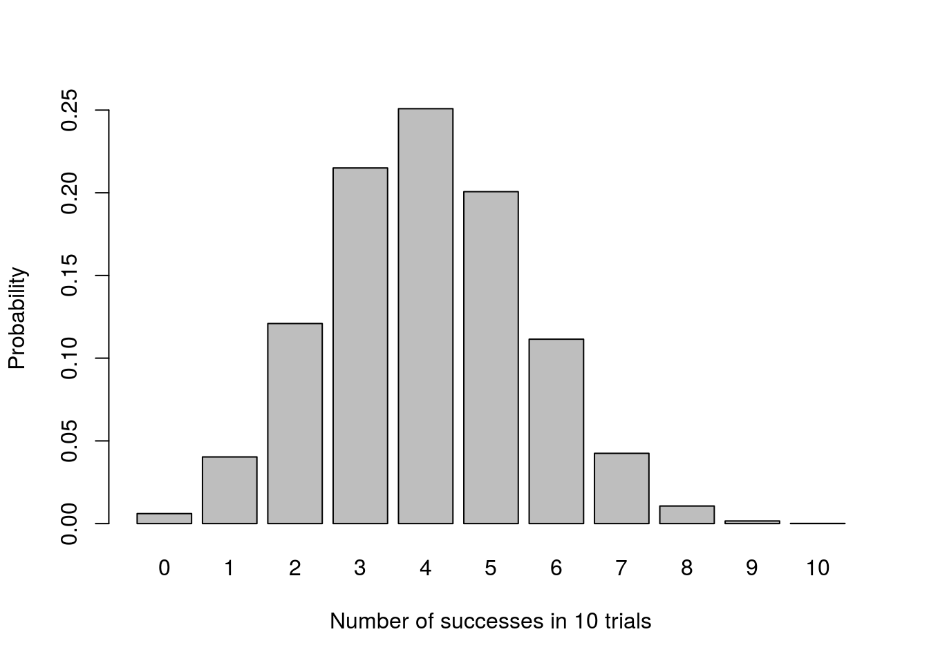

That looks sort of normal, though still a bit messy. What happens if we take a larger sample?

# Set new number of trials:
n <- 25

# initialize variable
pThisMany <- numeric()

for(k in 0:n){
  # Calculate p of this MANY successes
  pThisMany[as.character(k)] <-
    probSuccess^k * (1 - probSuccess)^(n - k) * choose(n, k)
}


# Plot
barplot(pThisMany,
        xlab = "Number of successes in 25 trials",
        ylab = "Probability")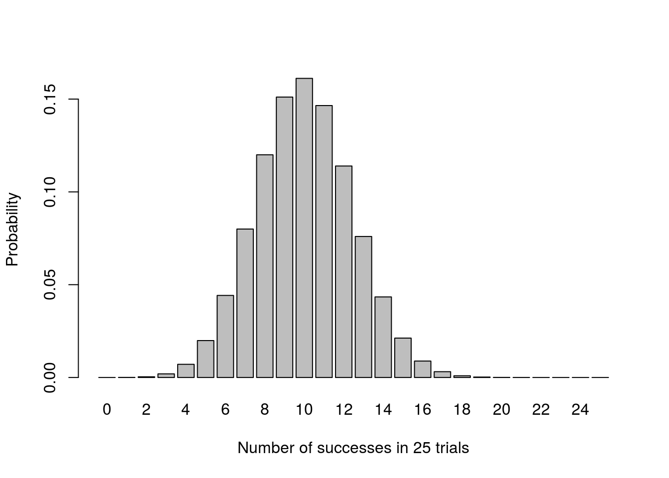

This plot looks very, very normal. Let’s see what happens if we do a sampling loop instead:

# initialize variable to hold number of successes
nSuccess <- numeric()

for(i in 1:12345){
  trials <- sample(c("points","no points"),
                   size = n,
                   replace = TRUE,
                   prob = c( probSuccess, 1 - probSuccess)
                   )
  
  nSuccess[i] <- sum(trials == "points" )
}

# Plot
hist(nSuccess)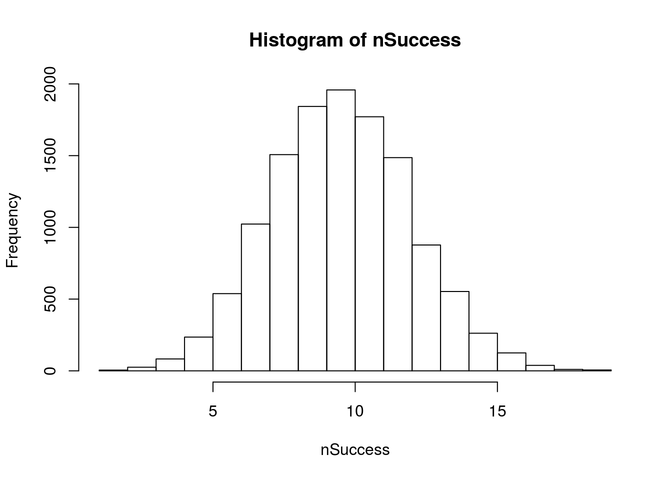

In fact, a normal curve should fit it just about perfectly.

hist(nSuccess, freq = FALSE)
curve(dnorm(x,
            mean=mean(nSuccess),
            sd = sd(nSuccess)),
      add = TRUE,
      col = "green3",
      lwd = 2)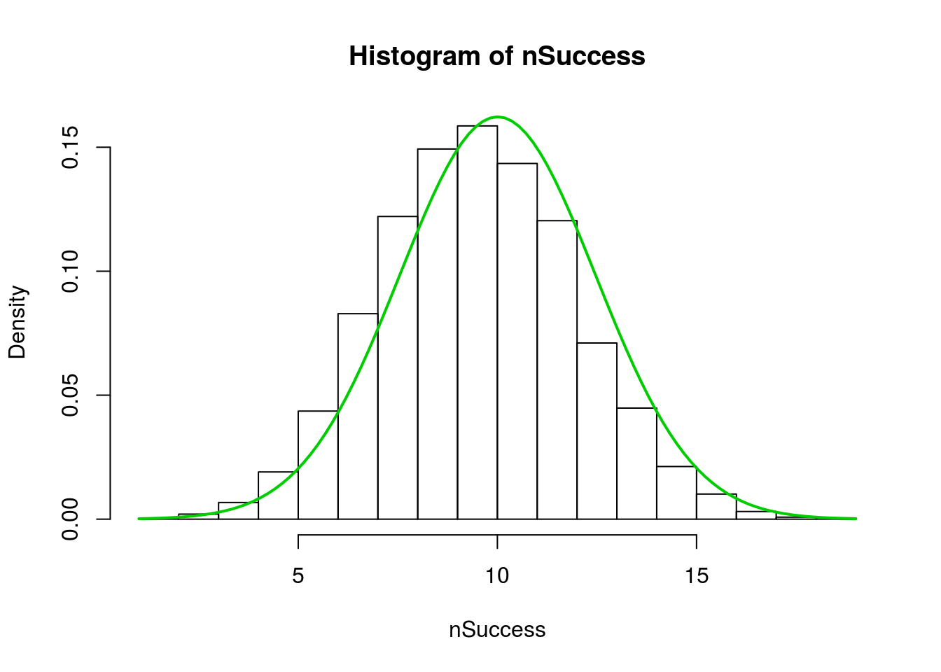

Note that, because each bin is the counts, the right hand edge of each bar is the true representation. A bit more playing can show that. This hist() sets the breaks at each “half” from just below zero to just above n. So, the center of each bar is now over its value.

hist(nSuccess,
     freq = FALSE,
     breaks = (0:(n+1)) - 0.5)
curve(dnorm(x,
            mean=mean(nSuccess),
            sd = sd(nSuccess)),
      add = TRUE,
      col = "green3",
      lwd = 2)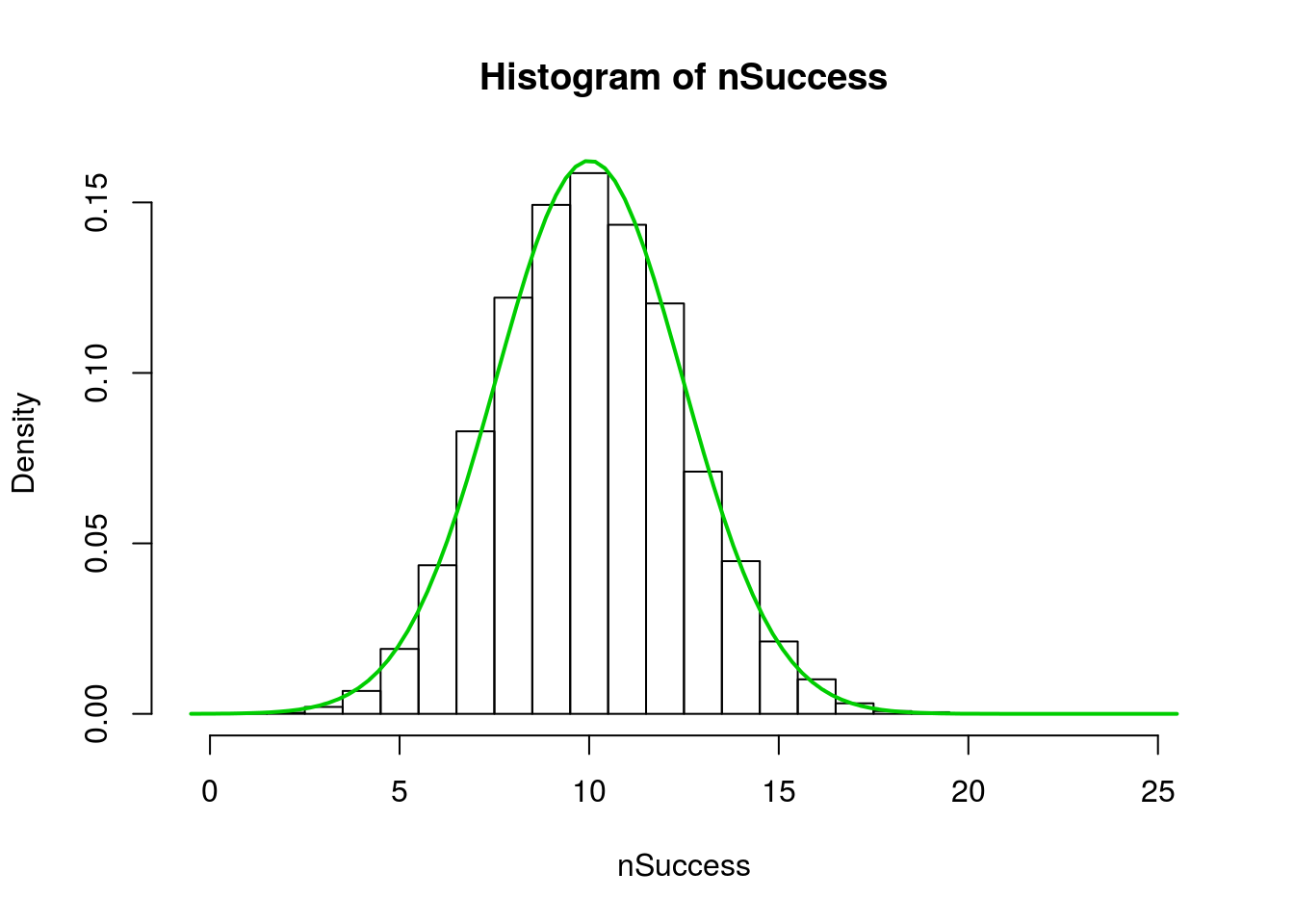

This should all look rather familiar. The sampling distribution is almost identical to what we did when doing bootstrap and null distributions for proportions. The only difference is that there we used mean() to calculate a proportion, and here we used sum() to calculate the number of successes instead. Dividing by our n will give us proportions instead:

hist(nSuccess/ n,
     breaks = 0:n/n)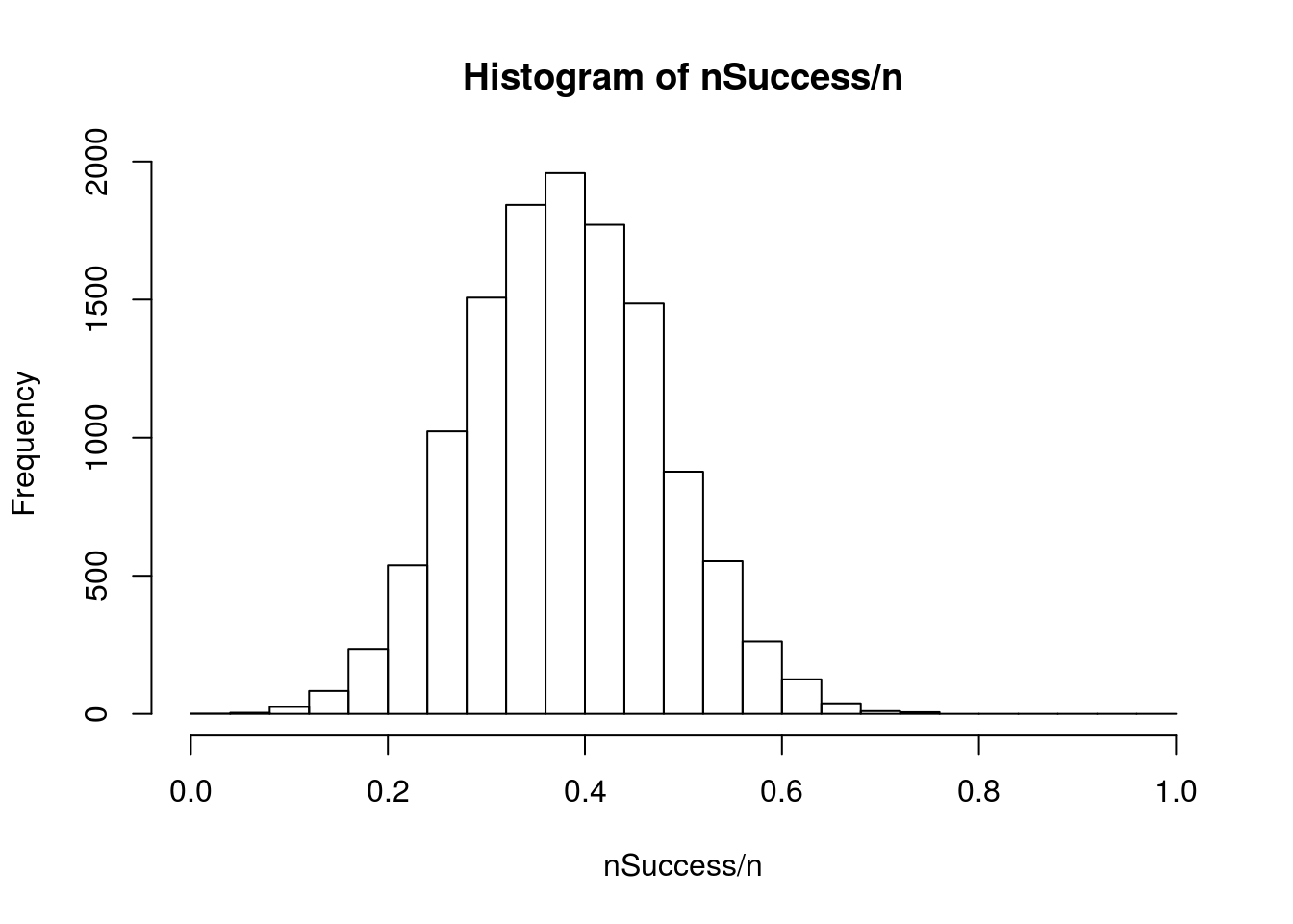

This is not a coincidence, and it turns out that the math that we relied on to get our shortcuts for Standard Error are based, in part, on understanding the underlying principles of the binomial systems.